AN EXTREME LEARNING MACHINE CLASSIFIER

FOR PREDICTION OF RELATIVE SOLVENT ACCESSIBILITY

IN PROTEINS

Saras Saraswathi, Andrzej Kloczkowski and Robert L. Jernigan

Department of Biochemistry, Biophysics and Molecular Biology

L. H. Baker Center for Bioinformatics and Biological Statistics, Iowa State University

112 Office and Laboratory Building, Ames, IA, 50011, U.S.A.

Keywords: Relative solvent accessibility, Support vector machine, Neural network, Extreme learning machine,

Prediction.

Abstract: A neural network based method called Sparse-Extreme Learning Machine (S-ELM) is used for prediction of

Relative Solvent Accessibility (RSA) in proteins. We have shown that multiple-fold gains in speed of

processing by S-ELM compared to using SVM for classification, while accuracy efficiencies are

comparable to literature. The study indicates that using S-ELM would give a distinct advantage in terms of

processing speed and performance for RSA prediction.

1 INTRODUCTION

Proteins perform a variety of important biological

functions that are imperative to the wellbeing of all

living things. Various factors determine protein

functions, such as, its native structure, the

information coded in its constituent amino acid

sequences, its reactions to the surrounding solvent

environment and the Relative Solvent Accessibility

(RSA) values of its residues and. Evaluating RSA

values will help to gain an insight into the structure

and function of a protein.

Protein structures and other related values such

as RSA can be experimentally determined by using

NMR spectroscopy or X-Ray crystallography. But

these methods can be expensive in terms of cost,

time and other factors. There is an urgent need to

process large amounts of data (spawned by advances

in biotechnology) accurately and speedily in order to

decipher the information buried in biological data,

since it is impractical to do it manually.

Computational methods such as machine learning

algorithms provide an alternate way by which we

can study this data in a cost and time efficient

manner. Still, accuracies and processing efficiencies

in existing methods are inadequate and there is a

need for improvement. This study endeavours to

attain a large gain in processing efficiencies.

RSA prediction has contributed to the study of

protein functions in many applications; to determine

protein hydration properties (Ooi, Oobatake,

Namethy, & Scheraga, 1987), identify temperature

sensitive residues that can be targeted for

mutagenesis and to study contact residue

information (Shen and Vihinen 2003), improve

secondary structure prediction (Adamczak, Porollo

& Meller, 2005) and for fold recognition and protein

domain (DOMpro) prediction (Cheng and Baldi,

2006). RSA values can be used to gauge degree of

solvent exposure of segments of globular proteins

(Carugo, 2003), to find residues with potential

structural or functional (ConSeq) importance

(Berezin, Glaser, Rosenberg, Paz, Pupko, Fariselli,

Casadio, & Ben-Tal, 2004), help with rationale

design of antibodies and other proteins to improve

binding affinities (David, Asprer, Ibana, Concepcion

& Padlan, 2007). In general RSA values can help to

achieve cost and time efficiencies in drug discovery

processes and help to gain a better understanding of

biological processes.

Probability profiles are used by Gianese, Bossa

& Pascarella (2003) to predict RSA values from

single sequence and Multiple Sequence Alignment

(MSA) data. Singh, Gromiha, Sarai & Ahmad

(2006) estimate RSA values from an atomic

perspective. Pollastri, Martin, Mooney & Vullo

364

Saraswathi S., Jernigan R. and Kloczkowski A..

AN EXTREME LEARNING MACHINE CLASSIFIER FOR PREDICTION OF RELATIVE SOLVENT ACCESSIBILITY IN PROTEINS .

DOI: 10.5220/0003086803640369

In Proceedings of the International Conference on Fuzzy Computation and 2nd International Conference on Neural Computation (ICNC-2010), pages

364-369

ISBN: 978-989-8425-32-4

 2010 SCITEPRESS (Science and Technology Publications, Lda.)

(2007) use homologous structural information to

improve RSA prediction. In addition, tertiary

structure predictions are increasingly being

augmented and improved with information derived

from secondary structure and RSA predictions.

Zarei, Arab & Sadeghi (2007) find that pairs of

residues can influence RSA prediction accuracy.

Knowledge-based tools which use machine

learning techniques and statistical theory can be

valuable in predicting RSA, especially in the

absence of evolutionary information or where

sequences are not well preserved. A number of

computational methods have been used for RSA

prediction, such as Neural Networks (NN) (Shandar

and Gromiha, 2002; Adamczak et al., 2005; Cheng,

Sweredoski, & Baldi, 2006; Huang, Zhu & Siew,

2006;). Pollastri, Baldi, Fariselli & Casadio (2002)

use RSA values of residues for scoring remote

homology searches and modelling protein folding

and structure using a bidirectional recurrent neural

network (ACCpro). Other methods include

Information Theory (Manesh, Sadeghi, Arab &

Movahedi, 2001), Multiple Linear Regression

Methods (Pollastri et al. 2002; Wagner et al. 2005),

Support Vector Machines (SVM) (Nguyen and

Rajapakse 2005) and fuzzy k-nearest neighbour

algorithm (Sim, Kim & Lee, 2005). Kim and Park

(2004) have used the SVMpsi and long range

interactions to improve RSA accuracy. Chen, Zhou,

Hu & Yoo (2004) compare five different methods,

decision tree (DT), Support Vector Machine (SVM),

Bayesian Statistics (BS), Neural Network (NN) and

Multiple Linear Regression (MLR) on the same data

set in order to compare the capabilities of different

methods in predicting RSA. They conclude that NN

and SVM are among the best methods for RSA

prediction.

More recently, Bondugula and Xu (2008)

combine sequence and structural information to

estimate RSA values (MUPRED) in order to predict

RSA. Petersen, Petersen, Andersen, Nielsen and

Lundegaard (2009) argue for the need of a reliability

score (Z-score) for measuring the degree of trust that

can be related to individual predictions. Meshkin

and Ghafuri (2010) use a two-step approach, using

feature selection on physico-chemical properties of

residues and Support Vector Regression (SVR) to

predict RSA.

We propose to use a new fairly new method

called Sparse Extreme Learning Machine (S-ELM),

based on neural networks, which is capable of

extreme speeds compared to traditional neural

networks while maintaining current classification

accuracies.

This paper is organized as follows. Section 2

briefly discusses the S-ELM algorithm and

characteristics of the RSA data. Section 3 discusses

the results of this study with performance

comparisons with SVM and NETASA methods

followed by conclusions in Section 4.

2 METHODS AND DATA

2.1 Extreme Learning Machine

Single Layer Feed-forward Network (SLFN), with a

hidden layer and an activation function possess an

inherent structure suitable for mapping complex

characteristics, learning and optimization. They have

applications in bioinformatics for solving various

problems like pattern classification and recognition,

structure prediction and data mining. The free

parameters of the network are learned from given

training samples using gradient descent algorithms

that are relatively slow and have many issues in

error convergence. A modified SLFN model called

an Extreme Learning Machine (ELM) has emerged

recently (Huang, Zhu, & Siew 2006), where it has

been proved theoretically that ELM can provide

good generalization performance and overcome

some of the problems associated with traditional

NNs such as stopping criterion, learning rate,

number of epochs and local minima. ELM has good

generalization capabilities and capacity to learn

extremely fast. The input weights are chosen

randomly but the output weights are calculated

analytically using a pseudo-inverse. Many activation

functions such as sigmoidal, sine, Gaussian or hard-

limiting functions can be used at the hidden layer

and the class is determined as the class which has

the maximum output value. A comprehensive

description of the S-ELM algorithm is given by

Huang et. al., (2006).

Even though the ELM algorithm requires less

training time, the random selection of input weights

affects the generalization performance when the data

is sparse or data is imbalanced. Suresh, Saraswathi

and Sundararajan (2010) and Saraswathi et al.

(2010) offer an improved version of ELM called the

Sparse-ELM (S-ELM) which gives better

generalization for sparse data. Hence, we use S-

ELM algorithm for predicting the RSA of proteins

where the imbalance in data varies with the different

threshold values used. S-ELM is also well suited for

RSA predictions of sequences whose structures have

not yet been determined and where there are no

homologs in existing sequences. The data is discus-

AN EXTREME LEARNING MACHINE CLASSIFIER FOR PREDICTION OF RELATIVE SOLVENT

ACCESSIBILITY IN PROTEINS

365

sed in detail in section 3.

We call the ELM algorithm for each of the

training data sets over several thresholds. We find

the optimal number of hidden neurons using a

unipolar sigmoidal activation function (lambda =

0.001) and perform K-fold (k = 5) validations. In K-

fold validation, the training set is separated into K-

groups. K-1 groups are used for training in each of

the K iterations and the model is tested on the

remaining K

group. The optimal parameters are

stored and used during the testing phase. The

performance of the S-ELM classifier and the time

taken to develop the RSA S-ELM classifier model is

compared with SVM using LIBSVM (Fan, Chen and

Lin, 2005) approach to show that the S-ELM

approach can achieve a slightly better performance

within a much shorter time. Five-fold cross

validation accuracies, processing time gains and

comparative studies are discussed in the results

section.

2.2 Data

Proteins consist of sequences of amino acid residues

that play a key role in determining the secondary and

tertiary structure of a protein. The sequential

relationship among the solvent accessibilities of

neighbouring residues can be used to improve the

results (although solvent accessibility is considered

evolutionarily less preserved than secondary

structure). We use binary values and a window size

of 8 to represent the amino acid sequences.

RSA of an amino acid residue is defined

(Mucchielli-Giorgi et al. 1999) as the ratio of the

solvent-accessible surface area of the residue

observed in the 3-D structure to that observed in an

extended tripeptide (Gly-X-Gly or Ala-X-Ala)

conformation. RSA is a simple measure of the

degree to which each residue in an amino acid

sequence is exposed to its solvent environment. For

our study, we consider the well-known Manesh data

set (Manesh, Sadeghi, Arab, & Movahedi, 2001)

which has a high imbalance with respect to the

number of samples per class (Table 1), where the

number of samples belonging to one class is much

lesser than the samples belonging to the other

classes.

The Manesh data set consists of 215 proteins, of

which 30 proteins (7545 residues) with variable

number of amino acid residues are used for classifier

model development and the remaining 185 proteins

(43137 residues) were used for evaluating the

generalization performance of the S-ELM classifier

through a 5-fold cross-validation model. The data in

the training and testing set are cast into two-class

and three-class problems (Table 1) by determining

whether the RSA value is below, between or above a

particular threshold. We use various % thresholds (0,

5, 10, 25, 50 for two-class and between 10_20 or

25_50 for three class), in order to compare our

results with those existing in literature. A residue is

considered as buried if its value is less than or equal

to the lower range, partially buried if it is between

the lower and the higher range and considered

exposed if its RSA value is higher than the range of

values (> 20 or > 50). The accuracy of the

predictions depend on the value of the thresholds

chosen and can vary widely with different residue

compositions in different proteins as discussed in the

results section.

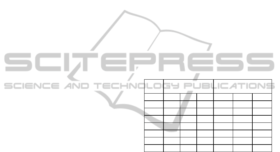
Table 1: Samples per class for 2-class and 3-class data

where thresholds are set between 0 and 50% for two class

(C0 and C1) and between 0, 10 and 50 % for 3-class (C0

C1 and C2).

Number of

Training residues

Number of

Testing residues

% C0 C1 C2 C0 C1 C2

0 867 6678 ** 4713 38424 **

5 5796 1749 ** 32943 10194 **

10 2826 4719 ** 15864 27273 **

20 4065 3480 ** 23111 20026 **

50 5796 1749 ** 32945 10192 **

10_20 3888 831 2826 22265 5008 15864

25_50 1750 1750 4065 10194 9832 23111

3 RESULTS AND DISCUSSION

We compare the results of our simulation using S-

ELM on the Manesh data set with the SVM

algorithm and NETASA (Shandar & Gromiha 2002)

methods (Figure 1 and Table 2), using the same set

of proteins for training and testing. Hence

comparisons with literature are made only with the

NETASA results.

The accuracy of the RSA predictions is measured

by the number of residues correctly classified as

belonging to class1 (E for exposed) for the two class

problem and as belonging to class2 (E) for the three

class problem. Prediction accuracy for training and

testing data sets is defined as the total number of

correctly predicted values for each class over the

total number of available residues in all classes. The

data shown in Table 2 indicates that the S-ELM

approach achieves a better accuracy for training and

testing than the corresponding results for the

ICFC 2010 - International Conference on Fuzzy Computation

366

NETASA paper. The SVM algorithm takes a longer

time to build the model as shown in Figure 2 and 3,

whereas the S-ELM algorithm process data at the

same speed for all combinations of data, showing

that the algorithm does not slow down when

complex data is involved. S-ELM uses optimal

parameters that are stored during the training phase

making it possible to run through the tests quickly.

Figure 1: Accuracy comparison between NETASA and S-

ELM, shows slight improvements for S-ELM method.

The training results for the SVM are between

89% and 99% for a range of thresholds. The

corresponding testing results saw gains for some of

the thresholds, while almost same results for the

others. The test results vary from 69% to 89% over a

range of thresholds, for the two class problem. The

results are much better for the S-ELM algorithm,

where the training and testing results are closer

together showing better generalization. The training

results vary between 73 % and 89% while the test

results vary between 71% and 89% which are better

than the results for the SVM and NETASA method.

Our interest in including the SVM in our simulations

was to show the advantages in time factor when the

S-ELM algorithm is used. The training results for

the S-ELM show a little gain over the NETASA and

the SVM results, but the testing results for S-ELM

clearly show higher results of between .006 to 4.476

% as seen in Figure 1 and Table 2. Similarly for the

three-class problem, seen on the last two lines of

Figure 3, the training accuracies for SVM are very

high at 99% while the testing accuracies are 68%

and 54% for two different thresholds, which are

slightly higher than for the NETASA results.

For the S-ELM results, the training accuracies

are closer to the testing accuracies, indicating better

generalization for the 3-class problem also. Here the

S-ELM test results show between 3 to 4% gains as

compared to the NETASA results. As indicated by

many results in the literature, the accuracies can vary

widely for different thresholds and different number

of classes into which the data is divided. A general

trend in the literature is that the RSA prediction

results vary between 70 % and 80%, similar to what

is seen here. So, the S-ELM gives comparable

results to literature.

Table 2: Training and Testing accuracies comparisons

between NETASA, SVM and S_ELM for all thresholds

using 350 hidden neurons are given. The support vectors

are given for SVM data.

NET-

ASA

SVM SVM S-ELM

Thres -

hold %

Accuracy %

Accuracy

for 350

hidden

neurons %

Training

0 89.8 99.9 3837 88.6

5 76.1 99.9 5894 79.8

10 75.2 99.9 6610 74.0

20 73.1 99.9 6826 72.98

50 80.1 99.9 5897 79.80

10 -20 65.1 99.9 7075 67.12

25 -50 60.9 99.9 7087 63.51

Testing

0 87.9 89.1 ** 89.1

5 74.6 76.2 ** 77.3

10 71.2 71.2 ** 73.1

20 70.3 69.5 ** 71.3

50 75.9 76.3 ** 77.3

10-20 63 64.1 ** 66.0

25-50 55 58.1 ** 59.5

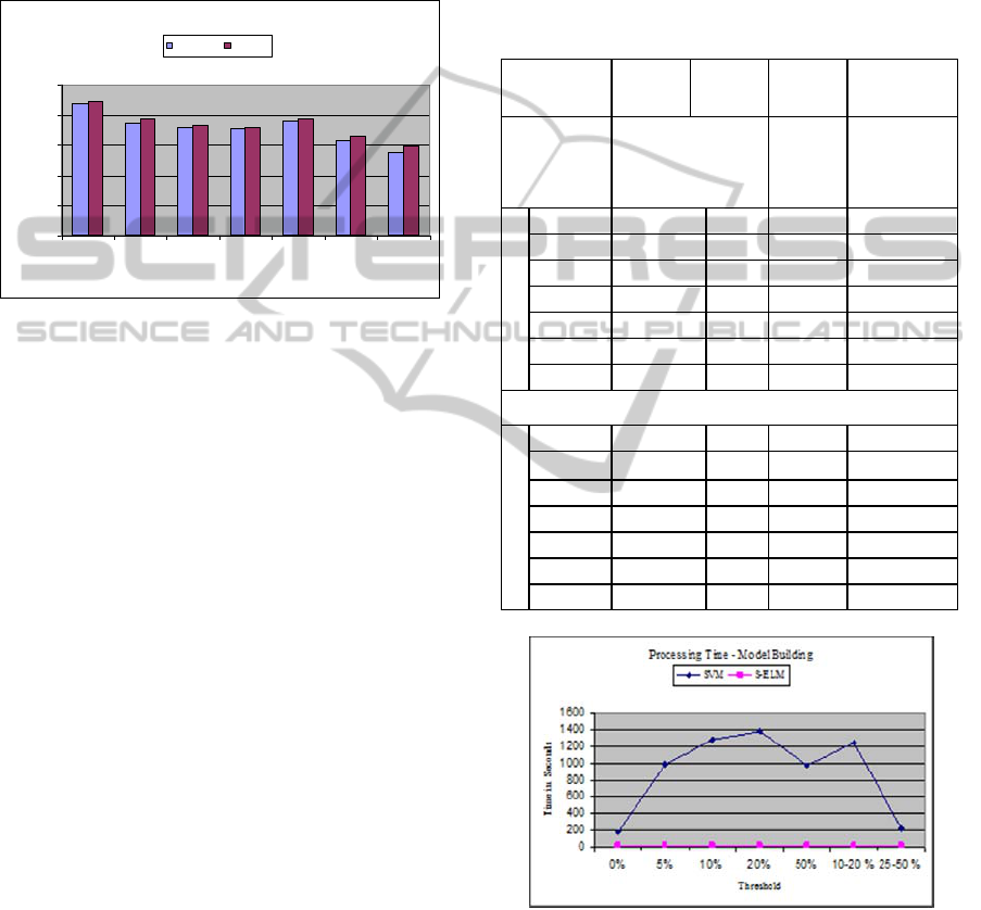
Figure 2: Processing time for modelling: SVM Vs. S-

ELM, clear shows huge gains in time for S-ELM.

The biggest advantage of using S-ELM comes

from the speed at which the data can be processed

by the algorithm, while providing us with slightly

better accuracies. It can be clearly seen from Table 3

that S-ELM has a clear advantage when it comes to

processing speed. The same number of samples of

Accuracy - NETASA Vs S-ELM

100

0% 5% 10% 20% 50% 10-20 % 25-50 %

Threshold

Accuracy %

NETASA S-ELM

AN EXTREME LEARNING MACHINE CLASSIFIER FOR PREDICTION OF RELATIVE SOLVENT

ACCESSIBILITY IN PROTEINS

367

7545 training sample residues was used for model

building for both algorithms. The ratio of time taken

by SVM and S-ELM for model building, for the

various thresholds range from 20.562 : 175 seconds

which amounts to almost 8.51 times time gain by S-

ELM for 0% threshold data. We find that the time

gains range from 8 times to multiple folds, the

highest being for the 20% threshold data where the

ratio is 20.562:1372.2 which is a gain of over 66.734

times. Generally, the time taken for model building

is most crucial, since the model needs to learn as

much as possible in the shortest time.

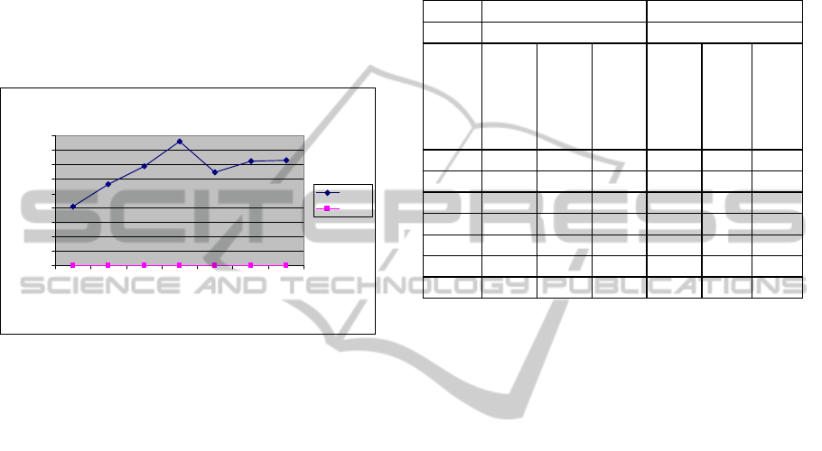
Figure 3: Processing time for testing: SVM Vs S-ELM.

For real time applications and for batch

processing applications it might be useful to have

faster testing capabilities and here we see that the S-

ELM algorithm is much faster in its testing

capabilities also. The same number of 43137 testing

residues was used here for the test runs in both

algorithms. Here the time gains between the testing

times for 0 % threshold is .922:410 which amounts

to 444.69 times fastr processing by S-ELM. We find

similar gains for other thresholds with the highest

gain for the 20% threshold at .937:857 which is

914.62 times faster processing speed. Both the SVM

and the S-ELM were run on the same computer

running XP windows operating system with 4 GB

RAM and Matlab software.

Time taken for training and testing runs by SVM

and S-ELM algorithms is given in Table 3. Figure 2

and Figure 3 illustrate the high processing time of

SVM and the very low and steady processing times

of S-ELM very clearly. The time taken by S-ELM is

very low at less than one or two seconds, shown as a

horizontal line close to the x-axis while the time

taken by SVM is quite high, ranging between 200

and 1400 seconds for training and between 400 and

900 seconds for testing. S-ELM takes very little time

for testing since stored optimal parameters are used

to calculate the output analytically using ELM.

There is no processing time data available to

compare speeds with the NETASA method. Future

studies will concentrate on increasing the accuracy

of S-ELM further using optimization techniques to

tune the S-ELM parameters for RSA prediction.

Table 3: Processing time for modelling, training and

testing: comparison between SVM and ELM.

SVM S-ELM

Time in Seconds Time in Seconds

Threshold %

Modelling

Training

Testing

Modelling

Training

Testing

0 175 24.6 410 20.6 0.5 0.92

5 990 105 561 20.8 0.6 0.94

10 1273 67 686 20.9 0.6 0.92

20 1372 76 857 20.9 0.5 0.94

50 977 89 645 20.9 0.6 0.95

10-20 1239 88 723 21.0 1.1 1.08

25-50 226 74 728 21.0 0.7 1.08

4 CONCLUSIONS

We have used the SVM and S-ELM methods of

classification for RSA prediction, using the Manesh

data set. We have compared the performance of

these algorithms with each other and with NETASA,

with respect to the speed of processing and have

shown that there are multiple-fold gains in

computational efficiency while using S-ELM

algorithm. It will be advantageous to use the S-ELM

algorithm for real time and batch processing

applications where accuracy and speed are equally

important.

ACKNOWLEDGEMENTS

We acknowledge the support of National Institutes

of Health through grants R01GM081680,

R01GM072014, and R01GM073095 and the support

of the NSF grant through IGERT-0504304.

REFERENCES

Adamczak, R., Porollo, A., & Meller, J. 2005. Combining

prediction of secondary structure and solvent

accessibility in proteins. Proteins, 59(3) 467-475.

Processing Time - Testing

100

200

300

400

500

600

700

800

900

0% 5% 10% 20% 50% 10-20

25-50

Threshold

Time in Seconds

SVM

S- E L M

ICFC 2010 - International Conference on Fuzzy Computation

368

Altschul, S., Madden, T., Schaffer, A., Zhang, J., Zhang,

Z., Miller, W., & Lipman, D., 1997. Gapped BLAST

and PSI-BLAST: a new generation of protein database

search programs. Nucleic Acids Res, 25(17) 3389-

3402.

Berezin, C., Glaser, F., Rosenberg, J., Paz, I., Pupko, T.,

Fariselli, P., Casadio, R., & Ben-Tal, N., 2004.

ConSeq: the identification of functionally and

structurally important residues in protein sequences.

Bioinformatics, 20, (8) 1322-1324.

Bondugula, R. & Xu, D., 2008. Combining Sequence and

Structural Profiles for Protein Solvent Accessibility

Prediction, In Comput Syst Bioinformatics ConfC,

195-202.

Carugo, O., 2003. Prediction of polypeptide fragments

exposed to the solvent. In Silico Biology, 3(4), 417-

428.

Chen, H., Zhou, H.-X., Hu, X., & Yoo, I., 2004

Classification Comparison of Prediction of Solvent

Accessibility from Protein Sequences, In 2nd Asia-

Pacific Bioinformatics Conference (APBC), 333-338.

Cheng, J., Sweredoski, M., & Baldi, P., 2006. DOMpro:

Protein Domain Prediction Using Profiles, Secondary

Structure, Relative Solvent Accessibility, and

Recursive Neural Networks. Data Mining and

Knowledge Discovery, 13(1) 1-10

Cortes, C. & Vapnik, V., 1995. Support vector networks.

Machine Learning, 20, 1-25.

David, M. P., Asprer, J. J., Ibana, J. S., Concepcion, G. P.,

& Padlan, E. A., 2007. A study of the structural

correlates of affinity maturation: Antibody affinity as a

function of chemical interactions, structural plasticity

and stability. Molecular Immunology, 44 (6), 1342-

1351.

Fan, R. E, Chen, P. H. and Lin, C. J., 2005. Working set

selection using second order information for training

SVM. Journal of Machine Learning Research, 6,

1889-1918.

Gianese, G., Bossa, F., & Pascarella, S., 2003.

Improvement in prediction of solvent accessibility by

probability profiles. Protein Engineering Design and

Selection, 16(12) 987-992.

Huang, G. B., Zhu, Q. Y., & Siew, C. K., 2006. Extreme

learning machine: Theory and applications.

Neurocomputing, 70, (1-3) 489-501

Kim, H. & Park, H., 2004. Prediction of protein relative

solvent accessibility with support vector machines and

long-range interaction 3D local descriptor. Proteins -

Structure, Function, and Bioinformatics, 54 (3), 557-

562.

Manesh, N. H., Sadeghi, M., Arab, S., & Movahedi, A. A.

M., 2001. Prediction of protein surface accessibility

with information theory. Proteins - Structure,

Function, and Genetics, 42 (4) 452-459.

Meshkin, A. & Ghafuri, H., 2010. Prediction of Relative

Solvent Accessibility by Support Vector Regression

and Best-First Method. EXCLI, 9, 29-38.

Mucchielli-Giorgi, M. H., Hazout, S., & Tuffery, P., 1999.

PredAcc: prediction of solvent accessibility.

Bioinformatics, 15 (2) 176-177.

Nguyen, M. N. & Rajapakse, J. C., 2005. Prediction of

protein relative solvent accessibility with a two-stage

SVM approach. Proteins, 59, (1) 30-37.

Ooi, T., Oobatake, M., Namethy, G., & Scheraga, H. A.,

1987. Accessible surface areas as a measure of the

thermodynamic parameters of hydration of peptides.

Proceedings of the National Academy of Sciences of

the United States of America, 84 (10) 3086-3090.

Petersen, B., Petersen, T. N., & Andersen , P., Nielsen,

M., Lundegaard, C., 2009. A generic method for

assignment of reliability scores applied to solvent

accessibility predictions. BMC Structural Biology,

9:51.

Pollastri, G., Baldi, P., Fariselli, P., & Casadio, R., 2002.

Prediction of coordination number and relative solvent

accessibility in proteins. Proteins, 47(2) 142-153.

Pollastri, G., Martin, A., Mooney, C., & Vullo, A., 2007.

Accurate prediction of protein secondary structure and

solvent accessibility by consensus combiners of

sequence and structure information. BMC

Bioinformatics, 8, (1) 201

Saraswathi, S., Suresh, S., Sundararajan, N., Zimmerman,

M. and Nilsen-Hamilton, M., 2010. ICGA-PSO-ELM

approach for Accurate Cancer Classification Resulting

in Reduced Gene Sets Involved in Cellular Interface

with the Microenvironment. IEEE Transactions in

Bioinformatics and Computational Biology,

http://www.computer.org/portal/web/csdl/doi/10.1109/

TCBB.2010.13.

Suresh, S., Saraswathi, S., Sundararajan, N., 2010.

Performance Enhancement of Extreme Learning

Machine for Multi-category Sparse Data Classification

Problems. Engineering Applications of Artificial

Intelligence,

http://dx.doi.org/10.1016/j.engappai.2010.06.009.

Shandar, A. & Gromiha, M. M., 2002. NETASA: neural

network based prediction of solvent accessibility.

Bioinformatics, 18(6), 819-824.

Shen, B. & Vihinen, M., 2003. RankViaContact: ranking

and visualization of amino acid contacts.

Bioinformatics, 19(16), 2161-2162.

Sim, J., Kim, S.-Y., & Lee, J., 2005. Prediction of protein

solvent accessibility using fuzzy k -nearest neighbor

method. Bioinformatics, 21(12), 2844-2849.

Singh, Y. H., Gromiha, M. M., Sarai, A., & Ahmad, S.,

2006. Atom-wise statistics and prediction of solvent

accessibility in proteins. Biophysical Chemistry,

124(2), 145-154.

Wagner, M., Adamczak, R., Porollo, A., & Meller, J.,

2005. Linear regression models for solvent

accessibility prediction in proteins. J Comput Biol,

12(3), 355-369.

Wang, J. Y., Lee, H. M., & Ahmad, S., 2007. SVM-

Cabins: prediction of solvent accessibility using

accumulation cutoff set and support vector machine.

Proteins, 68(1), 82-91.

Zarei, R., Arab, S., & Sadeghi, M., 2007. A method for

protein accessibility prediction based on residue types

and conformational states. Computational Biology and

Chemistry, 31(5-6) 384-388.

AN EXTREME LEARNING MACHINE CLASSIFIER FOR PREDICTION OF RELATIVE SOLVENT

ACCESSIBILITY IN PROTEINS

369