IMPROVED COMPRESSED GENETIC ALGORITHM: COGA-II

Kittipong Boonlong

Department of Mechanical Engineering, Burapha University 169 Long-Hard Bangsaen RoadTambon Saensook

Amphur Muang, Chonburi 20131, Thailand

Nachol Chaiyaratana

Department of Electrical Engineering, King Mongkut´s University of Technology North Bangok

1518 Pibulsongkram Road, Bangsue, Bangkok 10800, Thailand

Kuntinee Maneeratana

Department of Mechanical Engineering, Chulalongkorn University

Phayathai Road, Patumwan, Bangkok, 10330, Thailand

Keywords: Genetic algorithm, Multi-objective optimization, Objective compression.

Abstract: This paper presents an improved version of compressed objective genetic algorithm to solve problems with

a large number of objectives. The improved compressed objective genetic algorithm (COGA-II) employs a

rank assignment for the screening of non-dominated solutions that best approximate the Pareto front from

vast numbers of available non-dominated solutions. Since the winning non-dominated solutions are

heuristically determined from the survival competition, the procedure is referred to as a winning-score based

ranking mechanism. In COGA-II, an m-objective vector is transformed to only one criterion, the winning

score of which assignment is improved from that of the previous version, COGA. COGA-II is subsequently

benchmarked against a non-dominated sorting genetic algorithm II (NSGA-II) and an improved strength

Pareto genetic algorithm (SPEA-II), in seven scalable DTLZ benchmark problems. The results reveal that

for the closeness to the true Pareto front COGA-II is much better than NSGA-II, and SPEA-II. For diversity

of solutions, the diversity of the solutions by COGA-II is comparable to that of SPEA-II, while NSGA-II

has poor diversity. COGA-II can also prevent solutions diverging from true Pareto solutions that occur on

NSGA-II and SPEA-II for problems with more than 4 objectives. Thus, it can be concluded that COGA-II is

suitable for solving an optimization problem with a large number of objectives.

1 INTRODUCTION

In multi-objective optimization, an increase in the

number of conflicting objectives significantly raises

the difficulty level in multi-objective optimization

problems (Deb et al., 2005). The total number of

non-dominated solutions inevitably explodes owing

to the way that a non-dominated solution is defined.

When two candidate solutions are compared, a

solution a does not dominate another solution b

unless all objectives from a satisfy the domination

condition. With a large number of objectives, the

chance that two solutions cannot dominate one

another is unsurprisingly high. Since a genetic

algorithm is only capable of reporting a finite set of

solutions, a large number of possible non-dominated

solutions have to be screened for a good

approximation of Pareto front (Pierro et al., 2007,

Purshouse and Fleming, 2007)

This investigation also focuses on the screening

procedure that assigns “preference” levels to non-

dominated solutions in view that the higher the

preference level of non-dominated solutions, the

better the Pareto front approximation. A

compressed-objective genetic algorithm (COGA) is

an MOEA that successfully integrates this procedure

into the multi-objective search framework

(Maneeratana et al., 2006). The introduction of two

conflicting preference objectives during the

Boonlong K., Chaiyaratana N. and Maneeratana K..

IMPROVED COMPRESSED OBJECTIVE GENETIC ALGORITHM: COGA-II.

DOI: 10.5220/0003086700950103

In Proceedings of the International Conference on Evolutionary Computation (ICEC-2010), pages 95-103

ISBN: 978-989-8425-31-7

 2010 SCITEPRESS (Science and Technology Publications, Lda.)

competition between non-dominated solutions in

COGA transforms a three-or-more-objective

optimization problem into a two-objective problem.

This investigation also focuses on the screening

procedure that assigns “preference” levels to non-

dominated solutions in view that the higher the

preference level of non-dominated solutions, the

better the Pareto front approximation. A

compressed-objective genetic algorithm (COGA) is

an MOEA that successfully integrates this procedure

into the multi-objective search framework

(Maneeratana et al., 2006). The introduction of two

conflicting preference objectives during the

competition between non-dominated solutions in

COGA transforms a three-or-more-objective

optimization problem into a two-objective problem.

Here, a similar screening approach is introduced.

Instead of two conflicting preference objectives,

only one preference objective, a winning score, is

implemented. The winning score directly influences

the rank and hence survival chance of a solution.

With only one preference objective, the problem

representation transformation is simpler than that in

COGA. New MOEA with the winning score based

ranking mechanism is thus proposed: an improved

compressed-objective genetic algorithm (COGA-II).

COGA-II involves the assignment of preference

levels to non-dominated solutions for selection of

winning solutions that best describe the Pareto fronts

in problems with a large number of objectives. It is

benchmarked against the non-dominated sorting

genetic algorithm II, NSGA-II (Deb et al., 2002) and

the improved strength Pareto evolutionary

algorithm, SPEA-II (Zitzler et al., 2002). The chosen

test suites are DTLZ1-7 (Deb et al., 2005) with three

to six objectives. The organization of this paper is as

follows. In section 2, the proposed algorithm,

COGA-II is described. In section 3, the performance

evaluation criteria, covering an existing measure for

closeness to the Pareto front (Zitzler et al., 2000) and

a modified index for solution distribution, are

explained. Next, the results from benchmark trials

against NSGA-II, and SPEA-II are compared in

section 4 with the conclusions in section 5.

2 IMPROVED

COMPRESSED-OBJECTIVE

GENETIC ALGORITHM

Optimization problems usually arise when limited

resources are available for existing demands. If

multiple conflicting objectives are required in the

problem formulation, the problem is multi-objective.

Various techniques have been proposed for solving

these multi-objective problems. Among these, the

genetic algorithm has been established as one of the

most widely used methods for multi-objective

optimization (Li and Zhang 2006, Igel et al. 2007,

Zhou et al. 2007). Due to the parallel search nature

of the algorithm, the approximation of multiple

optimal solutions – the Pareto optimal solutions,

comprised of non-dominated individuals – can be

effectively executed. The performance of the

algorithm always degrades as the search space or

problem size gets bigger. An increase in the number

of conflicting objectives has also significantly raised

the difficulty level (Deb et al., 2005). Thus, the non-

dominated solutions may deviate from the true

Pareto front; the coverage of the Pareto front by the

solutions generated may be affected.

A number of strategies have been successfully

integrated into genetic algorithms to solve these

problems, including a direct modification of

selection pressure (Fonseca and Fleming, 1993),

(Srinivas and Deb, 1994) and elitism (Zitzler and

Thiele, 1999), (Keerativuttitumrong et al., 2002).

Although they have been proven to significantly

improve the search performance of genetic

algorithms, virtually all reported results deal with

only few objectives. In reality, the possibility that a

candidate solution is not dominated always increases

with objective numbers, leading to an explosion in

the total number of non-dominated solutions. This

difficulty stems from the way that a non-dominated

solution is defined. By domination definition, a

candidate solution x is dominated by another

solution y if and only if (a) all objectives from y are

either better than or equal to the corresponding

objectives from x and (b) at least one objective from

y is better than the corresponding objective from x.

Hence, if one single objective from y does not

satisfy the conditions, y would not dominate x. In a

problem with a large number of objectives, the

chance that two solutions cannot dominate one

another is inevitably high. A genetic algorithm must

be able to pick out a well chosen solution set from a

vast number of non-dominated solutions in order to

successfully approximate the Pareto front.

In order to properly approximate such Pareto

fronts, a number of non-dominated solutions must be

excluded from the search target. One possible

technique is to assign different preference levels to

non-dominated solutions under consideration. It is

hypothesized that a set containing highly preferred

solutions would reflect a close approximation of the

true Pareto front. The original compressed-objective

ICEC 2010 - International Conference on Evolutionary Computation

genetic algorithm (COGA) (Maneeratana et al.,

2006) employed two conflicting criteria in the

preference assignment. This can be viewed as a

transformation from an m-objective problem to a

two-objective problem during the survival

competition between two non-dominated solutions.

This thesis will present the improved version of

compressed-objective genetic algorithm. The

improved compressed objective genetic algorithm

(COGA-II) is quite different from the original

COGA in which three-or-more objectives is

transformed to only one preference objective during

the survival competition of two non-dominated

solutions. The preference objectives of the COGA

are winning score and vicinity index, in the other

hand, the COGA-II has only one preference

objective, winning score. Although the COGA-II

employs winning score as the COGA, its winning

score assignment is not the same as that of the

original algorithm. The winning score assignment of

and the main procedure of the COGA-II will be

described in the following topics.

2.1 Winning Score Assignment

The winning score is heuristically calculated from

the numbers of superior and inferior objectives

between a pair of two non-dominated individuals.

Let sup

, inj

and eq

be the number of objectives in

the individual i which are superior to the

corresponding objectives in the individual j, the

number of objectives in i which are inferior to that in

j, and the number of objectives in i which are equal

to that in j, respectively. For an objective k in an m-

objective problem, ρ

ijk

is defined as

⎪

⎩

⎪

⎨

⎧

ijijij

ijk

toequal is if 1,

oinferior t is if ,inf2/)inf(sup

osuperior t is if ,sup2/)inf(sup

(1)

The equation yields

∑

ijk

(2)

for any individual pairs i and j. The manner at

which ρ

ijk

deviates from one depends on the ratio

between the numbers of superior and inferior

objectives during each solution comparison. This

reflects the dependency and correlation among

objectives of interest.

Next, the summation of ρ

ijk

for the objective k

over all possible individual pairs is given by

∑∑

−

=+=

ijkk

(3)

where

N is the total number of non-dominated

individuals. The winning score of the individual i in

a non-dominated individual set or

is given by

∑

∑∑

lkk

ijkkij

iji

VVWF

qWFwwWS

/ and

, where,

(4)

The

ijk

is a competitive score. q

ijk

= 1 if the

objective

k of the individual i is superior to that of

the individual

j but q

ijk

= −1 if the objective k of i is

inferior to that of

j. Obviously, q

ijk

= 0 if the

objective

k from both individuals is equal. The w

a weighted sum of competitive scores from all

objectives. For any individual pair

i and j, w

= −w

= 0 and −1 < w

< 1. This leads to −N < WS

< N.

It is noted that the winning score assignment is not

an objectives weighted sum method such as Soylu

and Köksala (2010), Zhang and Li (2007). The

assignment is used for only non-dominated

solutions.

It is required that an individual with a high

winning score must be close to the true Pareto front.

This requirement is satisfied if the relationship

between the winning score and the distance from a

non-dominated individual to the true Pareto front in

the objective space can be described by a decreasing

function. This relationship can be identified using

the following multi-objective problem scenario.

Consider a multi-objective minimization problem in

which the

i-th objective or f

equals to the decision

variable

where x

∈ [0,1]. This problem has only

one true optimal solution with all objectives equal to

zero. First, a random solution is generated and

placed in an arc-hive. Another random solution is

then generated and compared with the archival

solution. The archive is appended if the new solution

is neither dominated by nor a duplicate of the

existing archival solution. At the same time, if the

new solution dominates the archival solution, the

dominated solution will be expunged from the

archive. The process of creating random solutions

and archive updating is repeated until the archive is

full.

Figure 1 displays the relationship between the

winning score of each solution and its distance to the

true optimal solution for problems with a different

number of objectives. The archive size is set to 200

while the illustrated problems contain 3–6, 8, 10, 15

and 20 objectives. In Figure 1, the relationship can

IMPROVED COMPRESSED GENETIC ALGORITHM: COGA-II

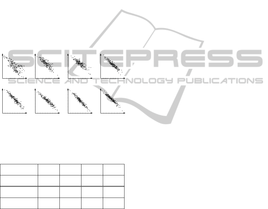
be described by a decreasing function especially

when the number of objectives is large.

Table 1 shows the average of percent correct

from comparison of all pairs of 200 non-dominated

solutions, of which the number of possible solution

pairs is equal to C(200,2) = (200!)/(198!2!) =

19,900, from 30 runs. For any solution pair

comparison, the comparison by winning score is

correct if the solution with a higher winning score is

closer to the true Pareto solution than the other. The

data in Table 1 show that winning score can

accurately identify different levels of the non-

dominated solution with more than 78% correctness

of comparison and its effectiveness is increased

when the number of objectives increases. Hence, the

winning score can be used to estimate the quality of

a solution in a non-dominated solution set.

3 objectives 4 objectives 5 objectives 6 objectives

8 objectives 10 objectives 15 objectives 20 objectives

Figure 1: Relationship between the winning score

(horizontal axis) and the distance from the true optimal

solution (vertical axis).

Table 1: Average of Percent Correct by Winning Score

Comparison of Various Numbers of Objectives.

No. of

Objectives

3 Obj 4 Obj 5 Obj 6 Obj

% Correct by

Winning Scores

78.08% 80.71% 85.60% 87.69%

No. of

Objectives

8 Obj 10 Obj 15 Obj 20 Obj

% Correct by

Winning Scores

89.82% 90.85% 91.55% 91.54%

2.2 Rank Assignment

With the use of the winning score, a rank value can

be assigned to an individual in COGA-II as follows.

1. Evaluate the winning score of each individual in

the non-dominated individual set.

2. Find extreme individuals among

N non-

dominated individuals. The number of extreme

individuals is equal to

E, which does not exceed

2m (two individuals with the minimum and

maximum values of each objective).

3. Sort

E extreme non-dominated individuals in

descending order of the winning score. The firstly

sorted individual is assigned rank 1. The secondly

sorted individual is assigned rank 2 and so forth.

Therefore, the lowest rank of extreme individuals

E. In the same way, N − E non-extreme non-

dominated individuals are also sorted in

descending order of the winning scores. However,

the ranks of these non-dominated individuals vary

from

E + 1 to N. This rank assignment guarantees

that a rank of an extreme individual is always

higher than that of a non-extreme individual.

4. Assign a rank to each dominated individual. The

rank of a dominated individual is given by

N plus

the number of its dominators. The addend

ensures that the rank of a non-dominated

individual is higher than that of a dominated

individual.

2.3 Main Procedure

The main algorithm for COGA-II is as follows.

1. Generate an initial population

and an empty

archive A

. Initialize the generation counter t = 0.

2. Merge the population

and the archival

population A

together to form the merged

population

. Then assign ranks to individuals in

3. Put all N non-dominated individuals from R

. into

the archive

t+1

. If N is larger than the archive

size Q, truncate the non-dominated individual set

using the operator described in the next sub-

section. On the other hand, if

N < Q then Q − N

dominated individuals with the least number of

their dominators are filled to the archive

t+1

4. Perform binary tournament selection with

replacement on archival individuals in order to

fill the mating pool with special attention to both

the rank and the summation of distances between

an individual

i or SDT

in the archive and all

individuals in the current mating pool.

At the beginning,

SDT

is set to zero. In the first

selection iteration, two individuals from the

archive are randomly picked; the individual with

higher rank will be selected. Otherwise, if their

ranks are equal, one individual is selected at

random. After the selection,

SDT

of any

remaining individual i in the archive is updated

by adding its current value with the distance

between the individual

i and the selected

individual. In the next selection iteration, the

winning individual is also determined from the

rank. However, if the ranks of two competing

individuals are equal, the individual with more

ICEC 2010 - International Conference on Evolutionary Computation

SDT

is selected. Subsequently, SDT

of an

individual i in the archive is again updated. The

binary tournament selection is then repeated until

the mating pool is fulfilled.

5. Apply crossover and mutation operations within

the mating pool. Then place the offspring into the

population P

t+1

and increase the generation

counter by one (t ← t + 1).

6. Go back to step 2 until the termination condition

is satisfied. Report the final archival individuals

as the output solution set.

A truncation operator for maintaining individuals

in the archive is introduced next.

2.4 Truncation

Only the winning score assignment may does not

guarantee diversity of solutions. The truncation is

therefore used to maintain the diversity of an archive

of any generation. With the use of the truncation

operator,

Q non-dominated individuals are extracted

from

N available individuals and placed into the

archive A

t+1

. The truncation operation is as follows

1. Find extreme individuals among

N non-

dominated individuals. The number of extreme

individuals is equal to

E, which does not exceed

m. If there is only one individual with the

minimum/maximum value of objective k, this is

the extreme individual. In contrast, if there are

multiple individuals with the minimum/maximum

value of objective

k, an individual is chosen at

random to be the extreme individual.

2. Place all

E extreme individuals in the archive. Set

the number of archival individuals L = E and

remaining individuals R = N − E. Then, calculate

the Euclidean distance

between the individual

i in R and its nearest neighbor in L. If there are

two-or-more individuals in L that have the same

objective vector as that of the individual j in

is set by

mcd

)1( −−=

(5)

3. Select

Q − L individuals with the highest values

from R. Then, move the candidate with the

highest winning score among these Q − L selected

individuals to the archive. If there are more than

one individual with the highest winning score, the

chosen candidate is the one with the highest value

4. Increase the counter for the number of archival

individuals (

L ← L + 1) and decrease the counter

for the number of remaining individuals (

R ← R –

1). Then, update

for the remaining individual i.

5. Go back to step 3 until the archive is fulfilled.

3 PERFORMANCE EVALUATION

CRITERIA

Good non-dominated solutions should be close to

the true Pareto front and uniformly distributed along

the front. From many available performance metrics

for MOEAs evaluation (Deb and Jain 2003), two

performance metrics are used here: the average

distance between the non-dominated solutions to the

true Pareto optimal solutions, or

metric (Zitzler

et al., 2002) and a newly proposed clustering index

CI for the description of solution distribution.

The clustering index CI is a diversity metric

which indicates the distribution of non-dominated

solutions on a hyper-surface. The proposed

differs from the grid diversity metric (Deb and Jain,

2002) such that the calculation of

CI does not

require a grid division of each objective, at which

the suitable number of divided grids is difficult to

identify.

For a non-dominated solution set

A of size Q, CI

of A is evaluated from a derived non-dominated

solution set

A' of size Q' where Q' >> Q. The

evaluation of CI from A is as follows from which the

range of

CI is between 0 and 1 where a higher CI

value indicates a better solution distribution. The CI

evaluation is as follows.

1. Copy all solutions in set

A to the derived solution

set A'.

2. Randomly select the first parent p

and parent p

from

A and A' respectively.

3. Perform crossover and mutation operations on

both parents to obtain two children

and c

Then, calculate objectives of both children.

4. Check whether each child neither dominates nor

is dominated by any solutions in

A. If both

children do not satisfy this condition, go back to

step 3. If only one child satisfies this condition,

put it in

A'; if both children satisfy the condition,

randomly pick a child and put it in

A'.

5. Update the number of members in A'. If A' is not

completely filled, go back to step 2. Otherwise,

go to step 7.

6. Divide

Q' solutions in A' into Q groups by a

clustering method [4]. Then, find the number of

groups

G that contains the first Q solutions,

which are identical to solutions in A. CI of A is

equal to

G/Q.

In this study, an acceptable value for Q', which

should be large as possible, is determined

IMPROVED COMPRESSED GENETIC ALGORITHM: COGA-II

empirically from all bench-mark problems and is

subsequently set at 4,000.

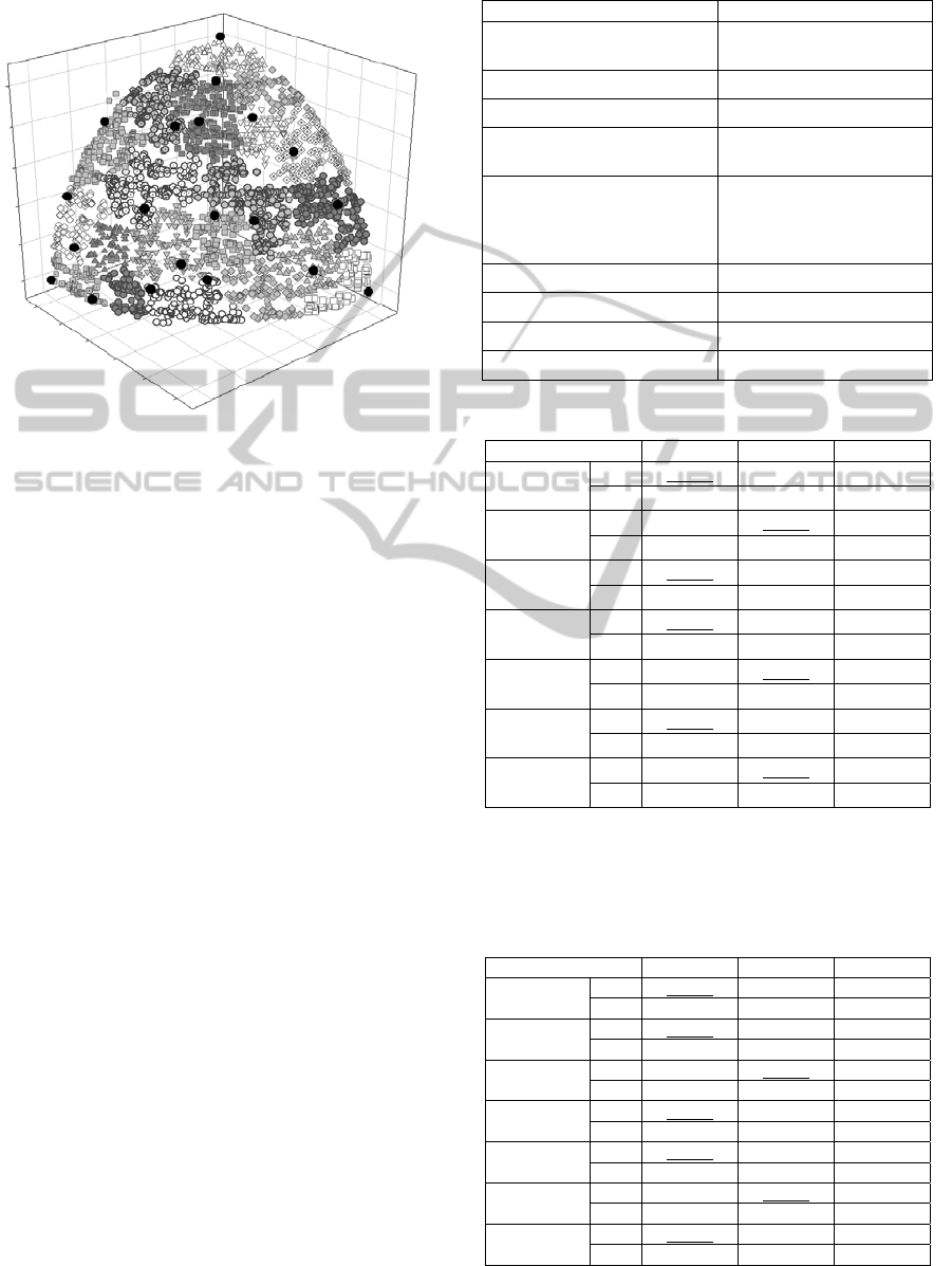
Figure 2: An example of CI evaluation of non-dominated

solutions from the three-objective DTLZ2.

The demonstration of CI calculation is given in

the following example in Figure 2. Let A contain 20

non-dominated solutions which are represented by

black circles of a three-objective DTLZ2 problem as

shown in the figure. After the derivation of

A' with

1,000 non-dominated solutions, solution clusters are

created. Each cluster is illustrated in the figure using

a unique marker.

CI is equal to the number of

clusters containing solutions from

A, 16, divided by

the total number of solutions in A, which is equal to

20. Thus, CI of A is equal to 0.80.

4 RESULTS AND DISCUSSIONS

COGA-II was compared against NSGA-II and

SPEA-II by the benchmark problems DTLZ1-7 with

3-6 objectives. The parameter setting is shown in

Table 2. The average (Avg.) and standard deviation

(SD) of

and CI are shown in Table 3 to Table 10.

From Table 3 to Table 10, COGA-II outperforms

NSGA-II and SPEA-II in terms of

. This

performance superiority is clearer with larger

numbers of objectives. In addition, the

performance of NSGA-II and SPEA-II is very close

to one another in the three-objective DTLZ1,

DTLZ2, DTLZ4 and DTLZ7 problems. However,

NSGA-II is better than SPEA-II once the number of

objectives increases. From the

CI values, the

performance of COGA-II and SPEA-II is quite

similar. In contrast, the performance of NSGA-II is

significantly worse than that of them.

Table 2: Parameter setting for NSGA-II, SPEA-II, and

COGA-II.

Parameter Setting and Values

Test Problems

DTLZ1-7 (Deb et al, 2005)

with |x

| = 10

Number of Objectives 3-6

Chromosome coding Real-value chromosome

Crossover method

SBX crossover (Deb, 2001)

with probability = 1.0

Mutation method

Variable-wise polynomial

mutation (Deb, 2001) with

probability = 1/number of

decision variables.

Population size 100

Archive size (except NSGA-II) 100

Number of generations 800

Number of repeated runs 30

Table 3: Summary of M

of DTLZ1-7 with 3 objectives.

Problem NSGA-II SPEA-II COGA-II

DTLZ1

Avg 0.0184

0.0197

0.0099

SD 0.0494 0.0392 0.0300

DTLZ2

Avg 0.0090 0.0089

0.0033

SD 0.0018 0.0014 0.0006

DTLZ3

Avg 0.0102

0.0324

0.0079

SD 0.0133 0.0521 0.0115

DTLZ4

Avg 0.0088

0.0094

0.0026

SD 0.0015 0.0018 0.0008

DTLZ5

Avg 0.0012 0.0010

0.0004

SD 0.0003 0.0003 0.0001

DTLZ6

Avg 0.0641

0.1269

0.0369

SD 0.0168 0.0331 0.0097

DTLZ7

Avg 0.0163 0.0162

0.0069

SD 0.0034 0.0026 0.0014

The number displayed in boldface is the best

result while the underlined number is the second

best result.

Table 4: Summary of M

of DTLZ1-7 with 4 objectives.

Problem NSGA-II SPEA-II COGA-II

DTLZ1

Avg 228.41

343.97

3.3139

SD 105.49 56.344 4.8817

DTLZ2

Avg 0.0395

0.0687

0.0054

SD 0.0120 0.0201 0.0015

DTLZ3

Avg 351.18 316.23

15.454

SD 59.885 49.012 10.236

DTLZ4

Avg 0.0416

0.1200

0.0043

SD 0.0204 0.0276 0.0018

DTLZ5

Avg 1.5054

1.5696

1.4583

SD 0.0643 0.0627 0.0751

DTLZ6

Avg 10.166 7.2514

4.6022

SD 0.6209 0.4098 0.4689

DTLZ7

Avg 0.1076

0.1082

0.0306

SD 0.0093 0.0136 0.0047

ICEC 2010 - International Conference on Evolutionary Computation

100

Table 5: Summary of M

of DTLZ1-7 with 5 objectives.

Problem NSGA-II SPEA-II COGA-II

DTLZ1

Avg

836.17

956.50

28.118

89.932 68.417 24.311

DTLZ2

Avg

0.4600

1.3523

0.0108

0.0987 0.1092 0.0034

DTLZ3

Avg

843.19

1024.7

254.63

96.118 88.152 68.619

DTLZ4

Avg

1.2253

1.5949

0.0054

0.2204 0.0742 0.0017

DTLZ5

Avg

2.2099

2.3259

2.1381

0.0863 0.1088 0.0593

DTLZ6

Avg

14.370

15.287

6.5050

0.2809 0.1743 0.3127

DTLZ7

Avg

0.2236

0.3917

0.0652

0.0328 0.0590 0.0078

Table 6: Summary of M

of DTLZ1-7 with 6 objectives.

Problem NSGA-II SPEA-II COGA-II

DTLZ1

Avg 1114.0

1230.98

161.84

SD 62.783 23.460 78.768

DTLZ2

Avg 1.6093

2.2346

0.0237

SD 0.1630 0.0308 0.0079

DTLZ3

Avg 1223.3 1674.4

482.55

SD 74.211 64.004 57.373

DTLZ4

Avg 1.9653 2.2703

0.0088

SD 0.0834 0.0268 0.0045

DTLZ5

Avg 3.2738

4.5426

2.5996

SD 0.2849 0.1072 0.0794

DTLZ6

Avg 19.451 20.362

10.495

SD 0.3376 0.2201 0.4016

DTLZ7

Avg 0.4441 0.9042

0.0836

SD 0.0664 0.1348 0.0127

Table 7: Summary of CI of DTLZ1-7 with 3 objectives.

Problem NSGA-II SPEA-II COGA-II

DTLZ1

Avg 0.5467

0.8420

0.8080

SD 0.0411 0.0816 0.0551

DTLZ2

Avg 0.5880

0.8967

0.8440

SD 0.0322 0.0234 0.0304

DTLZ3

Avg 0.5573 0.7673

0.7900

SD 0.0264 0.0571 0.0574

DTLZ4

Avg 0.6153

0.8847

0.8473

SD 0.0229 0.0249 0.0277

DTLZ5

Avg 0.7940

0.9200

0.8900

SD 0.0267 0.0174 0.0217

DTLZ6

Avg 0.6533 0.7833

0.8360

SD 0.0416 0.1088 0.0251

DTLZ7

Avg 0.5633

0.8340

0.8180

SD 0.0282 0.0243 0.0307

Table 8: Summary of CI of DTLZ1-7 with 4 objectives.

Problem NSGA-II SPEA-II COGA-II

DTLZ1

Avg 0.4053 0.7253

0.7847

SD 0.0588 0.0226 0.0646

DTLZ2

Avg 0.5213

0.8253

0.8220

SD 0.0352 0.0326 0.0250

DTLZ3

Avg 0.4720 0.7427

0.7800

SD 0.0509 0.0314 0.0638

DTLZ4

Avg 0.5513 0.7973

0.8067

SD 0.0415 0.0289 0.0192

DTLZ5

Avg 0.5007 0.7693

0.7913

SD 0.0284 0.0291 0.0252

DTLZ6

Avg 0.4980

0.7880

0.7587

SD 0.0300 0.0307 0.0249

DTLZ7

Avg 0.5400

0.8187

0.7747

SD 0.0270 0.0270 0.0344

Table 9: Summary of CI of DTLZ1-7 with 5 objectives.

Problem NSGA-II SPEA-II COGA-II

DTLZ1

Avg 0.4700

0.7400

0.7353

SD 0.0358 0.0507 0.0557

DTLZ2

Avg 0.4367 0.7780

0.8327

SD 0.0358 0.0351 0.0272

DTLZ3

Avg 0.4527 0.6813

0.7033

SD 0.0427 0.0310 0.0976

DTLZ4

Avg 0.4827 0.7867

0.8153

SD 0.0282 0.0270 0.0219

DTLZ5

Avg 0.4740

0.7620

0.7613

SD 0.0321 0.0313 0.0292

DTLZ6

Avg 0.5053

0.8880

0.7607

SD 0.0323 0.0175 0.0227

DTLZ7

Avg 0.5033

0.7793

0.7413

SD 0.0209 0.0347 0.0373

Table 10: Summary of CI of DTLZ1-7 with 6 objectives.

Problem NSGA-II SPEA-II COGA-II

DTLZ1

Avg 0.4740

0.8353

0.7627

SD 0.0478 0.0358 0.0432

DTLZ2

Avg 0.4653

0.8653

0.8320

SD 0.0426 0.0213 0.0316

DTLZ3

Avg 0.4413

0.8047

0.7420

SD 0.0240 0.0371 0.0448

DTLZ4

Avg 0.5077 0.8120

0.8147

SD 0.0233 0.0263 0.0273

DTLZ5

Avg 0.4340

0.8420

0.8113

SD 0.0228 0.0167 0.0326

DTLZ6

Avg 0.4973

0.8653

0.7593

SD 0.0221 0.0265 0.0353

DTLZ7

Avg 0.5157 0.7620

0.7727

SD 0.0327 0.0291 0.0307

IMPROVED COMPRESSED GENETIC ALGORITHM: COGA-II

101

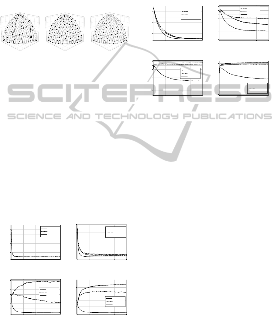
Figure 3 shows uniformity of solutions from a

run of DTLZ4 with 3 objectives from all algorithms.

Obviously, SPEA-II and COGA-II yeild more

diversity of solutions than NSGA-II. Figure 3 also

shows that solutions from COGA-II are quit well

uniform distribution.

(a) NSGA-II, CI

= 0.60

(a) SPEA-II, CI =

0.88

= 0.87

Figure 3: Examples of solutions from a run of DTLZ4

with 3 objectives of (a) NSGA-II, (b) SPEA-II, and

Graphs of average M

versus number of function

evaluations from all 30 runs from two selected

problems – DTLZ2 and DTLZ6 are shown in Figure

4 and Figure 5, respectively. All algorithms can

search solutions that are close to the true Pareto front

for the problems with 3 objectives with a close

convergence rate. However for the problems with 4

objectives, COGA-II clearly can search for solutions

with a better convergence rate. The performance of

COGA-II very obviously improves the NSGA-II and

SPEA-II when graphs of average

versus number

of function evaluations of the problems with 5-6

objectives are considered. Surprisingly, solutions

searched by NSGA-II and SPEA-II diverged from

the true Pareto front for the DTLZ2 with 6

objectives and DTLZ6 with 5 and 6 objectives if the

number of function evaluations is increased.

Number of Function Evaluation

0 20000 40000 60000 8000

Ave. Dist. to True Pareto Front

0.0

0.1

0.2

0.3

0.4

0.5

0.6

0.7

NSGA-II

SPEA-II

COGA-II

(a) DTLZ2 – 3 Objectives

Number of Function Evaluation

0 20000 40000 60000 8000

Ave. Dist. to True Pareto Front

0.0

0.2

0.4

0.6

0.8

NSGA-II

SPEA-II

COGA-II

(b) DTLZ2 – 4 Objectives

Number of Function Evaluation

0 20000 40000 60000 8000

Ave. Dist. to True Pareto Front

0.0

0.2

0.4

0.6

0.8

1.0

1.2

1.4

NSGA-II

SPEA-II

COGA-II

Number of Function Evaluation

0 20000 40000 60000 8000

Ave. Dist. to True Pareto Front

0.0

0.5

1.0

1.5

2.0

2.5

NSGA-II

SPEA-II

COGA-II

(d) DTLZ2 – 3 Objectives

Figure 4: Graphs of M

vs. Number of Function

Evaluations of DTLZ2 with 3-6 objecitves.

Therefore solutions obtained by the algorithms

are worse than solutions in the initial population.

This shows that Pareto domination alone is not

enough to solve problems with a large number of

objectives.

Number of Function Evaluation

0 20000 40000 60000 8000

Ave. Dist. to True Pareto Front

NSGA-II

SPEA-II

COGA-II

(a) DTLZ6 – 3 Objectives

Number of Function Evaluation

0 20000 40000 60000 8000

Ave. Dist. to True Pareto Front

NSGA-II

SPEA-II

COGA-II

(b) DTLZ6 – 4 Objectives

Number of Function Evaluation

0 20000 40000 60000 8000

Ave. Dist. to True Pareto Front

NSGA-II

SPEA-II

COGA-II

Number of Function Evaluation

0 20000 40000 60000 8000

Ave. Dist. to True Pareto Front

NSGA-II

SPEA-II

COGA-II

(d) DTLZ6 – 6 Objectives

Figure 5: Graphs of M

vs. Number of Function

Evaluations of DTLZ2 with 3-6 objecitves.

5 CONCLUSIONS

This paper presents COGA-II which integrates

preference notion into the process of non-dominated

solution screening for Pareto front approximation in

multi-objective problems with large number of

objectives. A criterion for selecting a winner from

the competition for survival between two non-

dominated solutions is thus defined. The proposed

ranking technique is referred to as a winning score

based ranking mechanism. The effectiveness of

COGA-II has been compared in benchmark trials

against those of NSGA-II and SPEA-II with multi-

objective DTLZ test problems. The performance

evaluation criteria are an average distance between

the non-dominated solutions and the true Pareto

front (

) [0] and a new clustering index (CI) for

solution distribution description. In overall, the

results indicate COGA-II are superior to NSGA-II

and SPEA-II in terms of the

index while the

solution distribution is comparable to that of SPEA-

II. COGA-II can also prevent solutions diverge from

true Pareto solution that occur on NSGA-II and

SPEA-II for problems with 5-6 objectives. Thus it

can conclude that COGA-II is suitable for solving an

optimization problem with large number of

objectives.

ICEC 2010 - International Conference on Evolutionary Computation

102

REFERENCES

Deb, K., 2001. “Multi-objective Optimization Using

Evolutionary Algorithms,” Chichester, UK: Wiley,

2001.

Deb, K., and Jain, S., 2002. “Running performance

metrics for evolutionary multi-objective optimization,”

in Proceedings of the Fourth Asia-Pacific Conference

on Simulated Evolution and Learning (SEAL’02),

Singapore, pp. 13–20.

Deb, K., Pratap, A., Agarwal, S., and Meyarivan, T., 2002.

“A fast and elitist multiobjective genetic algorithm:

NSGA-II,” IEEE Transactions on Evolutionary

Computation, vol. 6, no. 2, pp. 182–197.

Deb, K., Thiele L., Laumanns, M., and Zitzler, E., 2005.

“Scalable test problems for evolutionary multi-

objective optimization” in Evolutionary

Multiobjective Optimization: Theoretical Advances

and Applications, A. Abraham, L. C. Jain, and R.

Goldberg, Eds. London, UK: Springer, 2005, pp. 105–

145.

Fonseca, C. M.; and Fleming, P. J. 1993. “Genetic

algorithms for multi-objective optimization:

Formulation, discussion and generalization,”

Proceedings of the Fifth International Conference on

Genetic Algorithms, 416-423. Urbana-Champaign, IL,

USA.

Igel, C., Suttorp, T., and Hansen, N., 2007. “Steady-state

selection and efficient covariance matrix update in the

multi-objective CMA-ES,” Lecture Notes in Computer

Science, vol. 4403, pp. 171–185.

Keerativuttitumrong, N.; Chaiyaratana, N.; and Varavithya

V. 2002. “Multi-objective co-operative co-

evolutionary genetic algorithm,” Lecture Notes in

Computer Science. 2439: 288-297.

Li, H., and Zhang, Q., 2006. “A multiobjective differential

evolution based on decomposition for multiobjective

optimization with variable linkages,” Lecture Notes in

Computer Science, vol. 4193, pp. 583–592.

Maneeratana, K., Boonlong, K., and Chaiyaratana, N.,

2006. “Compressed-objective genetic algorithm,”

Lecture Notes in Computer Science, vol. 4193, pp.

473–482.

Pierro, F. D., Khu, S. T., and Savić, D. A.m 2007. “An

investigation on preference order ranking scheme for

multiojective evolutionary optimization,” IEEE

Transactions on Evolutionary Computation, vol. 11,

no. 1, pp. 17–45.

Purshouse, R. C. and P. J. Fleming, 2007. “On the

evolutionary optimization of many conflicting

objectives,” IEEE Transactions on Evolutionary

Computation, vol. 11, no. 6, pp. 770–784.

Soylu, B., and Köksala, M., “A favorable weight-based

evolutionary algorithm for multiple criteria problems”

2010. IEEE Transactions on Evolutionary

Computation, vol. 14, no. 2, pp. 191-205.

Srinivas, N.; and Deb, K. 1994. “Multi-objective function

optimization using non-dominated sorting genetic

algorithms,” Evolutionary Computation, 2(3): 221-

248.

Zhang, Q., and Li., H. 2007. “MOEA/D: A multiobjective

evolutionary algorithm based on decomposition”

IEEE Transactions on Evolutionary Computation, vol.

11, no. 6, pp. 712-731.

Zhou, A., Zhang, Q., Jin, Y,. and Sendhoff, B., 2007.

“Adaptive modelling strategy for continuous multi-

objective optimization,” in Proceedings of the 2007

Congress on Evolutionary Computation (CEC’07), pp.

431–437

Zitzler, E., Deb, K., and Thiele, L., 2000. “Comparison of

multiobjective evolutionary algorithms: Empirical

results,” Evolutionary Computation, vol. 8, no. 2, pp.

173–195.

Zitzler, E., Laumanns, M., and Thiele, L., 2002. “SPEA2:

Improving the strength Pareto evolutionary algorithm

for multiobjective optimization,” in Evolutionary

Methods for Design, Optimisation and Control, K.

Giannakoglou, D. Tsahalis, J. Periaux, K. Papailiou,

and T. Fogarty, Eds. Barcelona, Spain: CIMNE, pp.

95–100.

Zitzler, E., and Thiele, L. 1999. “Multiobjective

evolutionary algorithms: A comparative case study

and the strength Pareto approach,” IEEE

Transactions on Evolutionary Computation. 3(4): 257-

271.

IMPROVED COMPRESSED GENETIC ALGORITHM: COGA-II

103