TWO ALGORITHMS OF THE EXTENDED PSO FAMILY
Juan Luis Fern´andez-Mart´ınez
Energy Resources Department, Stanford University, Palo Alto, California, U.S.A.
Department of Civil and Environmental Engineering, University of California Berkeley, Berkeley, U.S.A.
Department of Mathematics, University of Oviedo, Oviedo, Spain
Esperanza Garc´ıa-Gonzalo
Department of Mathematics, University of Oviedo, Oviedo, Spain
Keywords:
Particle swarm optimization, Cloud algorithms, Stability analysis.
Abstract:
In this paper we present two novel algorithms belonging to the extended family of PSO: the PP-GPSO and the
RR-GPSO. These algorithms correspond respectively to progressive and regressive discretizations in acceler-
ation and velocity. PP-GPSO has the same velocity update than GPSO, but the velocities used to update the
trajectories are delayed one iteration, thus, PP-GPSO acts as a Jacobi system updating positions and velocities
at the same time. RR-GPSO is similar to a GPSO with stochastic constriction factor. Both versions have
a very different behavior from GPSO and the other family members introduced in the past: CC-GPSO and
CP-GPSO. The numerical comparison of all the family members has shown that RR-GPSO has the greatest
convergence rate and its good parameter sets can be calculated analytically since they are along a straight line
located in the first order stability region. Conversely PP-GPSO is a more explorative version.
1 INTRODUCTION
Particle swarm optimization (PSO) is a global
stochastic search algorithm used for optimization
motivated by the social behavior of individuals in
large groups in nature (Kennedy and Eberhart, 1995).
The particle swarm algorithm applied to optimization
problems is very simple: individuals, or particles, are
represented by vectors whose length is the number of
degrees of freedom of the optimization problem. To
start, a population of particles is initialized with ran-
dom positions (x
0
i
) and velocities (v
0
i
). A same objec-
tive function is used to compute the objective value
of each particle. As time advances, the position and
velocity of each particle is updated as a function of its
objective function value and of the objective function
values of its neighbors. At time-step k + 1, the algo-
rithm updates positions

x
k+1
i

and velocities

v
k+1
i

of the individuals as follows:
v
k+1
i
= ωv
k
i
+ φ
1
(g
k
− x
k
i
) + φ
2
(l
k
i
− x
k
i
),
x
k+1
i
= x
k
i
+ v
k+1
i
,
with
φ
1
= r
1
a
g
, φ
2
= r
2
a
l
,
r
1
,r
2
∈ U(0, 1) ω,a
l
,a
g
∈ R,
where l
k
i
is the i−th particle’s best position, g
k
the
global best position on the whole swarm, φ
1
, φ
2
are
the random global and local accelerations, and ω is a
real constant called inertia weight. Finally, r
1
and r
2
are random numbers uniformly distributed in (0,1),
to weight the global and local acceleration constants,
a
g
and a
l
.
PSO is the particular case for ∆t = 1 of the GPSO
algorithm (Fern´andez-Mart´ınez and Garc´ıa-Gonzalo,
2008):
v(t + ∆t) =(1− (1− ω)∆t)v(t)
+ φ
1
∆t(g(t)− x(t))+ φ
2
∆t(l(t) − x(t)),
x(t + ∆t) =x(t) + v(t + ∆t)∆t.
This model was derived using a mechanical anal-
ogy: a damped mass-spring system with unit mass,
damping factor,1− ω and total stiffness constant, φ =
φ
1
+ φ
2
, the so-called PSO continuous model:





x
′′
(t) +(1− ω) x
′
(t) +φx(t) = φ
1
g(t −t
0
) + φ
2
l(t −t
0
),
x(0) = x
0
,
x
′
(0) = v
0
,
t ∈ R.
(1)
Based on this physical analogy we were able to:
237
Luis Fernández-Martínez J. and Garcia-Gonzalo E..
TWO ALGORITHMS OF THE EXTENDED PSO FAMILY.
DOI: 10.5220/0003085702370242
In Proceedings of the International Conference on Evolutionary Computation (ICEC-2010), pages 237-242
ISBN: 978-989-8425-31-7
Copyright
c
 2010 SCITEPRESS (Science and Technology Publications, Lda.)

1. To analyze the PSO particle’s trajectories
(Fern´andez-Mart´ınez et al., 2008) and to explain-
ing the success in achieving convergence of some
popular parameters sets found in the literature
(Carlisle and Dozier, 2001), (Clerc and Kennedy,
2002), (Trelea, 2003).
2. To generalize PSO to any time step (Fern´andez-
Mart´ınez and Garc´ıa-Gonzalo, 2008), the so-
called Generalized Particle Swarm (GPSO). The
time step parameter has a physical meaning in
the mass-spring analogy but it is really a pseudo-
parameter in the optimization scheme that facili-
tates convergence.
3. To derive a family of PSO-like versions
(Fern´andez-Mart´ınez and Garc´ıa-Gonzalo,
2009), where the acceleration is discretized
using a centered scheme and the velocity of the
particles can be regressive (GPSO), progressive
(CP-GPSO) or centered (CC-GPSO). The consis-
tency of these algorithms have been explained in
terms of their respective first and second order
stability requirements. Although these regions are
linearly isomorphic, CC-GPSO and CP-GPSO
are very different from GPSO in terms of con-
vergence rate and exploration capabilities. These
algorithms have used to solve inverse problems
in environmental geophysics and in reservoir
engineering (Fern´andez-Mart´ınez et al., 2009),
(Fern´andez-Mart´ınez et al., 2010a), (Fern´andez-
Mart´ınez et al., 2010b), (Fern´andez-Mart´ınez
et al., 2010c).
4. To perform full stochastic analysis of the
PSO continuous and discrete models (GPSO)
(Fern´andez-Mart´ınez and Garc´ıa-Gonzalo,
2010b), (Fern´andez-Mart´ınez and Garc´ıa-
Gonzalo, 2010a). This analysis served to analyze
the GPSO second order trajectories, to show the
convergence of GPSO to the continuous PSO
model as the discretization time step goes to zero,
and to analyze the role of the oscillation center on
the first and second order continuous and discrete
dynamical systems.
In this contribution, following the same theoretical
framework we present two additional developments:
1. We introduce two other novel PSO-like meth-
ods: the PP-GPSO and the RR-GPSO (Garc´ıa-
Gonzalo and Fern´andez-Mart´ınez, 2009). These
algorithms correspond respectively to progressive
and regressive discretizations in acceleration and
velocity. PP-GPSO has the same velocity update
than GPSO, but the velocities used to update the
trajectories are delayed one iteration, thus, PP-
GPSO acts as a Jacobi system updating positions
and velocities at the same time. RR-GPSO is sim-
ilar to a GPSO with stochastic constriction factor.
Both versions have a very different behavior from
GPSO and the other family members introduced
in the past: CC-GPSO and CP-GPSO. RR-GPSO
seems to have the greatest convergence rate and
its good parameter sets can be calculated analyt-
ically since they are along a straight line located
in the first order stability region. Conversely PP-
GPSO seems to be a more explorative version, al-
though the behavior of these algorithms can be
partly problem dependent. Both exhibit a very pe-
culiar behavior, very different from other family
members, and thus they can be called distant PSO
relatives. RR-GPSO seems to have the greatest
convergence rate of all of them.
2. We present two different versions of the cloud
algorithms: the particle-cloud algorithm and the
coordinates algorithm that take adavantages from
the idea that GPSO, CC-GPSO and CP-GPSO op-
timizers are very consistent for a wide class of
benchmark functions when the PSO parameters
are close to the upper border of the second order
stability region. We show also that this situation
is slightly different for PP-GPSO and RR-GPSO.
2 THE IMMEDIATE PSO FAMILY
GPSO, CC-GPSO, CP-GPSO correspond to a cen-
tered discretization in acceleration and different
kind of discretizations in velocity (Fern´andez-
Mart´ınez and Garc´ıa-Gonzalo, 2009). Introducing a
β−discretization in velocity (β ∈ [0, 1]) :
x
′
(t) ≃
(β− 1)x(t − ∆t) + (1− 2β)x(t) + βx(t+ ∆t)
∆t
then, CP-GPSO corresponds to β = 1 (progressive),
CC-GPSO to β = 0.5 (centered) and GPSO to β = 0
(regressive). If ∆t = 1 they will be called PSO, CC-
PSO and CP-PSO respectively. The β-GPSO algo-
rithm can be written in terms of the absolute position
and velocity (x(t),v(t)) as follows:

x(t + ∆t)
v(t + ∆t)

= M
β

x(t)
v(t)

+ b
β
,
where
M
β1,1
= 1+ (β− 1)∆t
2
φ
M
β1,2
= ∆t(1+ (β− 1)(1− w)∆t)
M
β2,1
= ∆tφ
(1− β)β∆t
2
φ− 1
1+ (1− w)β∆t
M
β2,2
= (1− β∆t
2
φ)
1+ (1− w)(β− 1)∆t
1+ (1− w)β∆t
ICEC 2010 - International Conference on Evolutionary Computation
238

and
b
β1
= ∆t
2
(1− β)(φ
1
g(t − t
0
) + φ
2
l(t − t
0
))
b
β2
= ∆t
φ
1
(1−β)(1−β∆t
2
φ)g(t−t
0
)+βφ
1
g(t+∆t−t
0
)
1+(1−w)β∆t
+∆t
φ
2
(1−β)(1−β∆t
2
φ)l(t−t
0
)+φ
2
βl(t+∆t−t
0
)
1+(1−w)β∆t
The first and second order stability regions of the
β-GPSO depends on β (Fern´andez-Mart´ınez and
Garc´ıa-Gonzalo, 2009). Figure 1 shows the first
and second order stability regions with the associated
spectral radii for β = 0.75 and ∆t = 1 ( β-PSO). It
is similar to the CP-PSO case (β = 1) . In fact, when
0 ≤ β ≤ 0.5, the regions of first and second order sta-
bility are single domains, evolving from the GPSO to-
wards the CC-GPSO type, and when 0.5 < β ≤ 1 both
regions are composed of two zones, evolving towards
the CP-GPSO stability regions as β increases. The
¯
φ
!"#$! %&'$()*+,$-*./*$+0/1,*"2$*".)3+
$
$
4 5 4 65
7
8
9
5
9
8
7
:
5;6
5;9
5;<
5;8
5;4
5;7
5;=
5;:
5;>
6
¯
φ
!?#$! %&'$+/1-@.$-*./*$+0/1,*"2$*".)3+
$
$
4 5 4 65
7
8
9
5
9
8
7
:
5;9
5;<
5;8
5;4
5;7
5;=
5;:
5;>
6
Figure 1: First and second order stability regions for β-PSO
(β = 0.75) and associated spectral radius.
change of variables to make a β-GPSO version with
parameters a
g
, a
l
,w, ∆t, correspond to a standard PSO
(∆t = 1) with parameters b
g
, b
l
, and γ is:
b
g
=
∆t
2
1+ (1− w)β∆t
a
g
b
l
=
∆t
2
1+ (1− w)β∆t
a
l
γ =
1+ (1− w)(β− 1)∆t
1+ (1− w)β∆t
.
Good parameter sets are close to the upper limit
of second order stability (Fern´andez-Mart´ınez and
Garc´ıa-Gonzalo, 2009). Figure 2 shows for the
Griewank, Rosenbrock, Rastrigin and De Jong-f4
functions the median logarithmic error for 50 dimen-
sions, 100 particles, after 300 iterations and 50 runs
for a lattice of

ω,φ

points located on the GPSO first
stability region.
2.1 The Extended PSO Family
The PP-GPSO is derived by using progressive dis-
cretizations in acceleration and in velocity to approx-
imate the PSO continuous model (1):
ω
φ
(a) Griewank
−1 −0.5 0 0.5 1
0
0.5
1
1.5
2
2.5
3
3.5
4
−0.5
0
0.5
1
1.5
2
2.5
3
ω
φ
(b) Rosenbrock
−1 −0.5 0 0.5 1
0
0.5
1
1.5
2
2.5
3
3.5
4
3
4
5
6
7
8
ω
φ
(c) Rastrigin
−1 −0.5 0 0.5 1
0
0.5
1
1.5
2
2.5
3
3.5
4
2
2.1
2.2
2.3
2.4
2.5
2.6
2.7
2.8
ω
φ
(d) De Jong f4
−1 −0.5 0 0.5 1
0
0.5
1
1.5
2
2.5
3
3.5
4
−2
0
2
4
6
Figure 2: PSO: Mean error contourplot (in log
10
scale) for
the Griewank, Rosenbrock, Rastrigin and De Jong f4 func-
tions in 50 dimensions.
x
′
(t) ≃
x(t +∆t) − x(t)
∆t
x
′′
(t) ≃
x
′
(t + ∆t) − x
′
(t)
∆t
=
x(t +2∆t) − 2x(t +∆t) +x(t)
∆t
2
,
The following relationships apply:
x(t + ∆t) = x(t) + v(t)∆t,
v(t+∆t)−v(t)
∆t
+ (1− ω)v(t) =
φ
1
(g(t − t
0
) − x(t)) + φ
2
(l(t − t
0
) − x(t)).
Adopting t
0
= 0 we arrive at:
v(t +∆t) = (1− (1− ω) ∆t)v(t)
+φ
1
∆t(g(t) − x(t)) +φ
2
∆t(l(t) − x(t)),
x(t +∆t) = x(t) +v(t)∆t.
which has the same expression for the velocity that
the GPSO. The unique difference is that the velocity
used to update the trajectory is v(t) instead of v(t +∆t)
that is used in the GPSO. PP-PSO is the particular
case where the time step is ∆t = 1.
First and second order stability region can be de-
duced using the same methodology that in the other
family members (Fern´andez-Mart´ınez and Garc´ıa-
Gonzalo, 2009), that is, writting the first and second
order moments as dynamical systems and looking for
the region of the

ω,φ

plane where the eigenvalues
of the iterative matrix are on the unit circle.
Figure 3 shows the first and second order stability
regions of the PP-PSO case (∆t = 1) with the associ-
ated spectral radii. For the case of second order region
the parameter α has been set to 1 in this case. Both
regions of stability are bounded. The correspondence
TWO ALGORITHMS OF THE EXTENDED PSO FAMILY
239

¯
φ
!"#$%% %&'$()*+,$-*./*$+0/1,*"2$*".)3+
$
$
4 5 6 7 6
7
789
6
689
5
589
4
489
:
7
786
785
784
78:
789
78;
78<
78=
78>
6
¯
φ
!?#$%% %&'$&/1-@.$-*./*$+0/1,*"2$*".)3+
$
$
4 5 6 7
7
789
6
689
5
589
4
489
78:
789
78;
78<
78=
78>
6
Figure 3: PP-PSO: First and second order stability regions
and corresponding spectral radii.
between discrete trajectories for the GPSO and PP-
GPSO are:
ω
PSO
= ω
PP
+ ∆tφ
PP
,
φ
PSO
= φ
PP
.
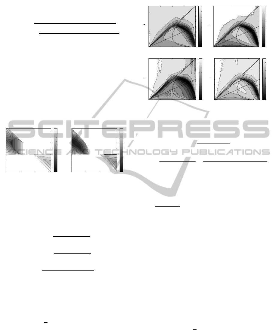
Figure 4 shows for the PP-PSO case the logarithmic
error for the Griewank, Rosenbrock, Rastrigin and De
Jong-f4 case for 50 dimensions, 100 particles, after
300 iterations and 50 runs. Compared to figure 2 it
can be observed that PP-PSO provides greater misfits
than the PSO, since PP-PSO updates at the same time
the velocities and positions of the particles. Also it
can be observed that the algorithm does not converge
for ω < 0, and the good parameter sets are in the com-
plex region (see figure 4) close to the limit of second
order stability and close to φ = 0. These results can
be partially altered when the velocities are clamped or
the time step is decreased.
3 RR-GPSO:
REGRESSIVE-REGRESSIVE
DISCRETIZATION
The PP-GPSO is derived by using regressive dis-
cretizations in acceleration and in velocity to approx-
imate the PSO continuous model (1) :
x
′
(t) ≃
x(t) − x(t − ∆t)
∆t
.
x
′′
(t) ≃
x
′
(t) − x
′
(t − ∆t)
∆t
=
x(t) − 2x(t − ∆t)+ x(t − 2∆t)
∆t
2
.
The following relationships apply:
x(t) = x(t − ∆t) +v(t)∆t,
v(t) − v(t − ∆t)
∆t
+ (1− ω)v(t) +φ(x(t − ∆t) +v(t)∆t) =
φ
1
g(t −t
0
) + φ
2
l(t −t
0
),
And we can express v(t) as:
ω
φ
(a) Griewank
−3 −2 −1 0
0
1
2
3
4
0.5
1
1.5
2
2.5
3
ω
φ
(b) Rosenbrock
−3 −2 −1 0
0
1
2
3
4
4.5
5
5.5
6
6.5
7
7.5
8
8.5
ω
φ
(c) Rastrigin
−3 −2 −1 0
0
1
2
3
4
2.1
2.2
2.3
2.4
2.5
2.6
2.7
2.8
ω
φ
(d) De Jong f4
−3 −2 −1 0
0
1
2
3
4
3
4
5
6
7
Figure 4: PP-PSO: Mean error contourplot (in log
10
scale)
for the Griewank, Rosenbrock, Rastrigin and De Jong f4
functions in 50 dimensions.
v(t) =
v(t − ∆t)+ φ
1
∆t(g(t − t
0
) − x(t − ∆t))
1+ (1− ω)∆t+φ∆t
2
+
φ
2
∆t(l(t − t
0
) − x(t − ∆t))
1+ (1− ω)∆t+φ∆t
2
.
The natural choice for t
0
is ∆t. Thus the RR-GPSO
algorithm with delay one becomes:
v(t +∆t) =
v(t) +φ
1
∆t(g(t) − x(t)) + φ
2
∆t(l(t) − x(t))
1+ (1− ω) ∆t+φ∆t
2
x(t +∆t) = x(t) +v(t + ∆t)∆t, t, ∆t ∈ R
x(0) = x
0
, v(0) = v
0
.
(2)
RR-GPSO with delay one is a particular case of (2)
for a unit time step, ∆t = 1. RR-GPSO is a PSO-like
algorithm where the parameter
A(ω,φ,∆t) =
1
1+ (1− ω)∆t+φ∆t
2
could be interpreted as a similar constriction factor
to this introduced by Clerc and Kennedy (Clerc and
Kennedy, 2002).
Figure 5 shows for ∆t = 1 (RR-PSO case) and
α = 1 (a
g
= a
l
), the first and second order stability
regions with the corresponding first and second or-
der spectral radii. Both regions of stability are un-
bounded. Also in both cases the first and second or-
der spectral radii are zero at the infinity:

ω,φ

=
(−∞,+∞) and

ω,φ

= (+∞,−∞). The correspon-
dence between discrete trajectories for the GPSO and
RR-GPSO are:
ω
PSO
=
ω
RR
− ∆tφ
RR
+ (1− ω
RR
)∆t + ∆t
2
φ
RR
1+ (1− ω
RR
)∆t + ∆t
2
φ
RR
,
φ
PSO
=
φ
RR
1+ (1− ω
RR
)∆t + ∆t
2
φ
RR
.
ICEC 2010 - International Conference on Evolutionary Computation
240

ω
¯
φ
(a) RR−PSO First order spectral radius
−10 −5 0 5
−10
−8
−6
−4
−2
0
2
4
6
8
0.3
0.4
0.5
0.6
0.7
0.8
0.9
1
ω
φ
(b) RR−PSO Second order spectral radius
−10 −5 0 5
−10
−8
−6
−4
−2
0
2
4
6
8
0.2
0.3
0.4
0.5
0.6
0.7
0.8
0.9
1
Figure 5: RR-PSO: First and second order stability regions
and corresponding spectral radii.
!"#$%&'(
φ
)
)
* + , - .
*
+
,
-
.
/*
/+
+
/
*
/
+
0
123$'4"25(
φ
)
)
* + , - .
*
+
,
-
.
/*
/+
0
,
6
-
7
.
1&38"#9#'
φ
)
)
* + , - .
*
+
,
-
.
/*
/+
*:6
/
/:6
+
+:6
;$)<2'9 =,
φ
)
)
* + , - .
*
+
,
-
.
/*
/+
-
,
+
*
+
,
-
Figure 6: RR-PSO: Mean error contourplot (in log
10
scale)
for the Griewank, Rosenbrock, Rastrigin and De Jong f4
functions in 50 dimensions.
The good parameters sets for the RR-PSO are con-
centrated around the line φ = 3(ω − 3/2), mainly for
inertia values greater than two (figure 6). This line is
the same for both functions and seems to be invariant
when the number of parameters increase. This result
is very different from the ones shown for the other
version, since the good parameters are not in relation
with the second order stability upper border. This line
is located in a zone of medium attenuation and high
frequency of trajectories. This last property allows
for a very efficient and explorative search around the
oscillation center of each particle in the swarm.The
theoretical and numerical results shown for different
PSO family members share the following observa-
tions:
1. The PSO algorithms perform fairly well for a very
broad region of inertia and total mean accelera-
tion. This region is close for all PSO members to
the upper limit of the second order stability region
for PSO, CC-PSO, CP-PSO and PP-PSO. For RR-
PSO the good points are along a straight line lo-
cated in a zone of medium attenuation and high
frequency of trajectories.
2. These regions are fairly the same for different
kind of benchmark functions. This means that the
same

ω,φ

points can be used to optimize a wide
range of cost functions.
Based on this idea we have designed a PSO algorithm
where each particle in the swarm has different inertia
(damping) and local and global acceleration (rigidity)
constants, being the

ω,φ

sets located in the low mis-
fit regions. This idea has been implemented for the
particle-cloud PSO algorithm and extended for CC-
PSO and CP-PSO.
The particle-cloud algorithm works as follows:
1. The misfit contours to design the clouds are based
on the Rosenbrock function in 50 dimensions.
The Rosenbrock function was chosen since in in-
verse problems the equivalent models that fit the
observed data within the same tolerance are lo-
cated on flat valleys.
2. For each

ω,φ

located on the low misfit region,
we generate three different (ω,a
g
,a
l
) points cor-
responding to a
g
= a
l
, a
g
= 2a
l
and a
l
= 2a
g
. Par-
ticles are randomly selected depending on the iter-
ations. The algorithm keep track of the (ω,a
g
,a
l
)
points used to achieve the global best solution
in each iteration. Thus, when these clouds are
used to optimize other benchmark functions with
lower complexity, the variability associated to
these points might be damped adequately using
the time step parameter (∆t).
It was shown that the criteria used to select the points
belonging to the cloud it is not very rigid, since points
located on the low misfit region (those that close to the
second order convergence border) provide very good
results, especially those that lie inside the complex
zone of the first order stability region. Also, adding
some popular parameter sets found in the literature
(Carlisle and Dozier, 2001), (Clerc and Kennedy,
2002), (Trelea, 2003) did not improve the results.
Table 1 shows the results obtained for different
benchmark functions in 50 dimensions, 100 particles,
300 iterations for 50 runs, using the particle cloud al-
gorithm. The misfits are compared in to the refer-
ence values calculated with the program published by
Birge (Birge, 2003). It can be observed that the CC-
PSO and PSO are the most performing algorithms for
all the benchmark functions except for the Rastrigin
case. In all the cases the misfits are similar or even
better than those presented in the literature. Never-
theless, as pointed before, in inverse modeling it is not
only important to achieve very low misfits but also to
explore the space of possible solutions. When these
algorithms have to be used in explorative form the
cloud versions become a very interesting approach,
because there is no need to tune the PSO parameters.
TWO ALGORITHMS OF THE EXTENDED PSO FAMILY
241

Table 1: Comparison between the particle-cloud modalities
and the reference misfit values found in the literature (Birge,
2003) for different benchmark functions in 50 dimensions.
Median Griewank Rastrigin Rosenbrock Sphere
Standard PSO 9.8E-03 81 90 6.9E-11
PSO 9.6E-03 92 86 8.9E-19
CC-PSO 7.4E-03 99 90 1.0E-15
CP-PSO 1.8E-02 86 223 2.0E-07
PP-PSO 1.0E-01 91 251 8.4E-02
RR-PSO 1.2E-02 39 89 2.9E-25
4 CONCLUSIONS
In this paper we present two more different members
of the PSO family: the PP-GPSO and the RR-GPSO.
Both versions are deduced from the PSO continuous
model adopting respectively a progressive and a re-
gressive discretization in velocities and accelerations.
Although they are PSO-like versions, PP-GPSO has
the same velocity update than GPSO and RR-GPSO
has the form of a PSO with constriction factor, its be-
havior is very different from the PSO case. Particu-
larly the the best parameters sets of the RR-PSO are
concentrated along a straight line located in the com-
plex zone of the first order stability region, but are
not in direct relation with the upper limit of the sec-
ond order stability zone. This behavior is very differ-
ent from others family members including PP-PSO.
The numerical comparison between all the members
of the PSO family using their corresponding cloud-
algorithmshas shown that RR-PSO has a veryimpres-
sive convergence rate while PP-PSO is a more explo-
rative version.
REFERENCES
Birge, B. (2003). PSOt - a particle swarm optimization tool-
box for use with Matlab. In Swarm Intelligence Sym-
posium, 2003. SIS ’03. Proceedings of the 2003 IEEE,
pages 182–186.
Carlisle, A. and Dozier, G. (2001). An off-the-shelf PSO.
In Proceedings of the Particle Swarm Optimization
Workshop, pages 1–6, Indianapolis, Indiana, USA.
Clerc, M. and Kennedy, J. (2002). The particle swarm -
explosion, stability, and convergence in a multidimen-
sional complex space. IEEE Transactions on Evolu-
tionary Computation, 6(1):58–73.
Fern´andez-Mart´ınez, J. L. and Garc´ıa-Gonzalo, E. (2008).
The generalized PSO: a new door to PSO evolu-
tion. Journal of Artificial Evolution and Applications,
2008:1–15.
Fern´andez-Mart´ınez, J. L. and Garc´ıa-Gonzalo, E. (2009).
The PSO family: deduction, stochastic analysis and
comparison. Swarm Intelligence, 3(4):245–273.
Fern´andez-Mart´ınez, J. L. and Garc´ıa-Gonzalo, E. (2010a).
Handbook of Swarm Intelligence –Concepts, Princi-
ples and Applications, chapter What makes Particle
Swarm Optimization a very interesting and powerful
algorithm? Adaptation, Learning and Optimization.
Springer.
Fern´andez-Mart´ınez, J. L. and Garc´ıa-Gonzalo, E. (2010b).
Stochastic stability analysis of the linear continuous
and discretePSO models. Technical report, Depart-
ment of Mathematics. University of Oviedo. Submit-
ted to IEEE Transactions on Evolutionary Computa-
tion.
Fern´andez-Mart´ınez, J. L., Garc´ıa-Gonzalo, E., and
Fern´andez-
´
Alvarez, J. (2008). Theoretical analysis of
particle swarm trajectories through a mechanical anal-
ogy. International Journal of Computational Intelli-
gence Research, 4(2):93–104.
Fern´andez-Mart´ınez, J. L., Garc´ıa-Gonzalo, E., Fern´andez-
´
Alvarez, J. P., Kuzma, H. A., and Men´endez-P´erez,
C. O. (2010a). PSO: A powerful algorithm to solve
geophysical inverse problems. application to a 1D-
DC resistivity case. Jounal of Applied Geophysics,
71(1):13–25.
Fern´andez-Mart´ınez, J. L., Garc´ıa-Gonzalo, E., and Naudet,
V. (2010b). Particle Swarm Optimization applied to
the solving and appraisal of the streaming potential
inverse problem. Geophysics. Accepted for publica-
tion.
Fern´andez-Mart´ınez, J. L., Kuzma, H. A., Garc´ıa-Gonzalo,
E., Fern´andez-D´ıaz, J. M., Fern´andez-
´
Alvarez, J.,
and Men´endez-P´erez, C. O. (2009). Application of
global optimization algorithms to a salt water intru-
sion problem. Symposium on the Application of Geo-
physics to Engineering and Environmental Problems,
22(1):252–260.
Fern´andez-Mart´ınez, J. L., Mukerji, T., and Garc´ıa-
Gonzalo, E. (2010c). Particle Swarm Optimization in
high dimensional spaces. In 7th International Confer-
ence on Swarm Intelligence (ANTS 2010), Brussels,
Belgium.
Garc´ıa-Gonzalo, E. and Fern´andez-Mart´ınez, J. L. (2009).
The PP-GPSO and RR-GPSO. Technical report, De-
partment of Mathematics. University of Oviedo. Sub-
mitted to IEEE Transactions on Evolutionary Compu-
tation.
Kennedy, J. and Eberhart, R. (1995). Particle swarm op-
timization. In Proceedings IEEE International Con-
ference on Neural Networks (ICNN ’95), volume 4,
pages 1942–1948, Perth, WA, Australia.
Trelea, I. (2003). The particle swarm optimization algo-
rithm: convergence analysis and parameter selection.
Information Processing Letters, 85(6):317 – 325.
ICEC 2010 - International Conference on Evolutionary Computation
242