A BIASED RANDOM KEY GENETIC ALGORITHM APPROACH

FOR UNIT COMMITMENT PROBLEM

Lu´ıs A. C. Roque

ISEP-DEMA/GECAD, Instituto Superior de Engenharia do Porto, Porto, Portugal

Dalila B. M. M. Fontes

FEP/LIAAD-INESC Porto L.A., Universidade do Porto, Porto, Portugal

Fernando A. C. C. Fontes

FEUP/ISR-Porto, Universidade do Porto, Porto, Portugal

Keywords:

Unit commitment, Genetic algorithm, Optimization, Electrical power generation.

Abstract:

A Biased Random Key Genetic Algorithm (BRKGA) is proposed to ﬁnd solutions for the unit commitment

problem. In this problem, one wishes to schedule energy production on a given set of thermal generation units

in order to meet energy demands at minimum cost, while satisfying a set of technological and spinning reserve

constraints. In the BRKGA, solutions are encoded by using random keys, which are represented as vectors

of real numbers in the interval [0, 1]. The GA proposed is a variant of the random key genetic algorithm,

since bias is introduced in the parent selection procedure, as well as in the crossover strategy. Tests have

been performed on benchmark large-scale power systems of up 100 units for a 24 hours period. The results

obtained have shown the proposed methodology to be an effective and efﬁcient tool for ﬁnding solutions to

large-scale unit commitment problems. Furthermore, form the comparisons made it can be concluded that the

results produced improve upon the best known solutions.

1 INTRODUCTION

The Unit Commitment (UC) problem is well known

in the power industry and adequate solutions for it

have the potential to save millions of dollars per year

in fuel and related costs. Therefore, the UC problem

plays a key role in planning and operation of power

systems. The UC problem is a complex decision mak-

ing process since it entails the schedule of the turn-on

and turn-off of the thermal generation units, as well

as the amount of power to be generated by each on-

line unit for each period of the generation horizon. In

addition, there are multiple technological constraints

and spinning reserveconstraints that must be satisﬁed.

Due to its combinatorial nature, multi-period charac-

teristics, and nonlinearities this problem is computa-

tionally demanding and, thus, no exact optimization

method is capable of solving the UC problem for real-

sized systems. In the past, several traditional heuristic

approaches based on exact methods have been used,

see e.g. (Lee, 1980; Cohen and Yoshimura, 1983;

Merlin and Sandrin, 1983). However, more recently

most of the developed methods are metaheuristics,

evolutionary algorithms, and hybrids of the them,

see e.g. (Arroyo and Conejo, 2002; Valenzuela

and Smith, 2002; Jenkins and Purushothama, 2003;

Dudek, 2004; Simopoulos et al., 2006; Chen and

Wang, 2007; Maturana and Riff, 2007; Senjyu et al.,

2008; Viana et al., 2008; Abookazemi et al., 2009).

These latter types have, in general lead to better

results than the ones obtained with the traditional

heuristics. Comprehensive and detailed surveys can

be found in (Padhy, 2001; Salam, 2007; Raglend and

Padhy, 2008).

In this paper we focus on applying Genetic Algo-

rithms (GAs) to ﬁnd good quality solutions for the UC

problem. The majority of the reported GA implemen-

tations to address the UC problem are based on the

binary encoding. However, studies have shown that

other encoding schemes such as real valued random

332

A. C. Roque L., B. M. M. Fontes D. and A. C. C. Fontes F..

A BIASED RANDOM KEY GENETIC ALGORITHM APPROACH FOR UNIT COMMITMENT PROBLEM.

DOI: 10.5220/0003076703320339

In Proceedings of the International Conference on Evolutionary Computation (ICEC-2010), pages 332-339

ISBN: 978-989-8425-31-7

 2010 SCITEPRESS (Science and Technology Publications, Lda.)

keys (Bean, 1994) can be efﬁcient when accompa-

nied with suitable GA operators, specially for prob-

lems where the relative order of tasks is important.

In the proposed algorithm a solution is encoded as

a vector of n real random keys in the interval [0,1],

where n is the number of generation units. The Bi-

ased Random Key Genetic Algorithm (BRKGA) pro-

posed in this paper is based on the framework pro-

vided by Resende and Gonc¸alves in (Gonc¸alves and

Resende, 2009). BRKGAs are a variation of the Ran-

dom key Genetic Algorithms (RKGAs), ﬁrst intro-

duced by Bean (Bean, 1994). The bias is introduced

at two different stages of the GA. On the one hand,

when parents are selected we get a higher change of

good solutions being chosen, since one of the parents

is always taken from a subset including the best so-

lutions. On the other hand, the crossover strategy

is more likely to choose alleles from the best par-

ent to be inherited by offspring. In (Gonc¸alves and

Resende, 2009) is presented a tutorial on the imple-

mentation and use of biased random key genetic algo-

rithms for solving combinatorial optimization prob-

lems and many successful applications are reported

in the references therein.

This paper is organized as follows. In Section 2,

the UC problem is described and formulated, while in

Section 3 the genetic algorithm proposed is explained.

Section 4 presents the set of benchmark systems used

in the computational experiments and reports on the

results obtained. Finally, in Section 5 some conclu-

sions are drawn.

2 UC PROBLEM FORMULATION

In the UC problem one needs to determine the turn-

on and turn-off times of the power generation units,

as well as the generation output subject to opera-

tional constraints, while satisfying load demands at

minimum cost. Therefore, we have two types of de-

cision variables. The binary variables, which indi-

cate the status of each unit in each time period and

the real variables, which provide the information on

the amount of energy produced by each unit in each

time period. The choices made must satisfy two sets

of constraints: the demand constraints, regarding the

load requirements and the spinning reserve require-

ments and the technical constraints, regarding gener-

ation units constraints. The costs are made up two

components: the fuel costs, i.e. production costs, and

the start-up costs.

Let us now introduce the parameters and decision

variables notation.

Yth

t, j

: (Thermal) Generation of unit j at time period

t, in [MW];

t, j

: Status of unit j at time period t (1 if the unit is

on; 0 otherwise);

T: Number of time periods (hours) of the scheduling

time horizon;

N: Number of generation units;

t: Time period index;

j: Generation unit index;

: Load demand at time period t, in [MW];

: System spinning reserve requirements at time

period t, in [MW];

Yth

Min/Max

: Minimum/maximum generation limits,

in [MW];

∆

dn/up

: maximum allowed output level de-

crease/increase in consecutive periods for

unit j, in [MW].

on/of f

min, j

: Minimum uptime/downtime of unit j, in

[hours];

on/of f

(t): Time periods for which unit j has been

continuously on-line/off-line until time period t,

in [hours];

c, j

: Number of time periods needed to cool down

unit j, in [hours];

H/C, j

: Hot/Cold start-up cost of unit j, in [$];

2.1 Objective Function

As already said, there are two cost components: gen-

eration costs and start-up costs. The generation costs,

i.e. the fuel costs, are conventionally given by a

quadratic cost function as in equation (1), while the

start-up costs, that depend on the number of time pe-

riods during which the unit has been off, are given as

in equation (2).

th, j

) = a

· (Yth

t, j

)

+ b

·Yth

t, j

+ c

, (1)

where a

are the cost coefﬁcients of unit j.

t, j

(

H, j

of f

min, j

≤ T

of f

(t) ≤ T

c, j

C, j

of f

(t) > T

c, j

. (2)

where SU

H, j

and SUS

C, j

are the hot and cold start-up

costs of unit j, respectively.

Therefore, the cost incurred with an optimal

scheduling is given by the minimization of the total

A BIASED RANDOM KEY GENETIC ALGORITHM APPROACH FOR UNIT COMMITMENT PROBLEM

333

costs for the whole planning period, as in equation

(3).

Minimize

∑

t=1

∑

j=1

(Yth

t, j

) · u

t, j

(3)

+SU

t, j

· (1− u

t−1, j

) · u

t, j

}

2.2 Constraints

The constraints can be divided into two sets: the de-

mand constraints and the technical constraints. Re-

garding the ﬁrst set of constraints it can be further

divided into load requirements and spinning reserve

requirements, which can be written as follows:

1. Power Balance Constraints. The total power

generated must meet the load demand, for each time

period.

∑

j=1

Yth

t, j

· u

t, j

≥ D

,t ∈ {1,2,...,T}. (4)

2. Spinning Reserve Constraints. The spinning

reserve is the total amount of real power generation

available from on-line units net of their current pro-

duction level.

∑

j=1

Yth

max, j

· u

t, j

≥ Dr

+ D

,t ∈ {1,2,...,T}. (5)

The second set of constrains includes unit output

range, minimum number of time periods that the unit

must be in each status (on-line and off-line), and the

maximum output variation allowed for each unit.

3. Unit Output Range Constraints. Each unit has

a maximum and minimum production capacity.

Yth

min, j

· u

t, j

≤ Yth

t, j

≤ Yth

max, j

· u

t, j

, (6)

for t ∈ {1, 2, ...,T} and j ∈ {1,2,...,N}.

4. Ramp Rate Constraints. Due to the thermal

stress limitations and mechanical characteristics the

output variation levels of each online unit in two con-

secutive periods are restricted by ramp rate limits.

−∆

≤ Yth

t, j

−Yth

t−1, j

≤ ∆

, (7)

for t ∈ {1, 2, ...,T} and j ∈ {1,2,...,N}.

5. Minimum Uptime/Downtime Constraints. The

unit cannot be turned on or off instantaneously once

it is committed or uncommitted. The minimum up-

time/downtime constraints indicate that there will be

a minimum time before it is shut-down or started-up,

respectively.

(t) ≥ T

min, j

and T

of f

(t) ≤ T

of f

min, j

, (8)

for t ∈ {1, 2, ...,T} and j ∈ {1, 2, ..., N}.

3 BIASED RANDOM KEY

GENETIC ALGORITHM

Genetic Algorithms (GAs) are a optimization tech-

nique based on natural genetics and evolution mech-

anisms such as survival of the ﬁttest law, genetic

recombination and selection (Holland, 1975; Gold-

berg, 1989). GAs provide great modeling ﬂexibility

and can easily be implemented to search for solu-

tions of combinatorial optimization problems. Sev-

eral GAs have been proposed for the unit commit-

ment problem, see e.g. (Kazarlis et al., 1996; Cheng

et al., 2000; Swarup and Yamashiro, 2002; Arroyo

and Conejo, 2002; Xing and Wu, 2002; Dudek, 2004;

Abookazemi et al., 2009), the main differences be-

ing the representation scheme, the decoding proce-

dure, and the solution evaluation procedure (i.e. ﬁt-

ness function).

Many GA operators have been used; the most

common being copy, crossover, and mutation. Copy

consists of simply copying the best solutions from the

previous generation into the next one, with the inten-

tion of preserving the chromosomes corresponding to

best solutions in the population. Crossover produces

one or more offsprings by combining the genes of so-

lutions chosen to act as their parents. The mutation

operator randomly changes one or more genes of a

given chromosome in order to introduce some extra

variability into the population and thus, prevent pre-

mature convergence.

The GA proposed here, i.e. the BRKGA, uses

the framework proposed by Resend and Gonc¸alves

in (Gonc¸alves and Resende, 2009). The algorithm

evolves a population of chromosomes that are used to

assign priorities to the generation units. These chro-

mosomes are vectors, of size N (number of units),

of real numbers from the interval [0, 1] (called ran-

dom keys). A new population is obtained by joining

three subsets of solutions as follows: the ﬁrst subset

is obtained by copying the best solutions of the cur-

rent population; the second subset is obtained by us-

ing a (biased) parameterized uniform crossover; the

remaining solutions, termed mutants, are randomly

ICEC 2010 - International Conference on Evolutionary Computation

334

generated as was the case for the initial population.

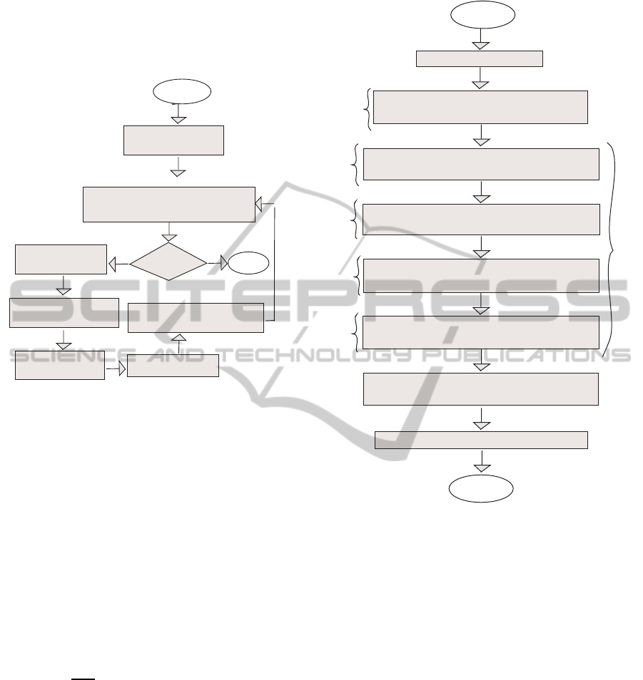
The BRKGA framework is illustrated in Figure 1,

which has been adapted from (Gonc¸alves and Re-

sende, 2009).

Entry

Generation of

random key vectors

Decoding: Random keys vectors in

terms of the generation scheduling

All

generations?

Exit

Sort chromosomes

by fitness value

Classify chromosomes

as elit or non-elite

Copy elite

chromosomes

Generate mutants

Combine elite and non- elite

to produce offspring

Figure 1: The BRKGA framework.

Speciﬁc to our problem is the decode and repair

procedure, that is how solutions are constructed once

a population of chromosomes is given. The decoding

procedure is performed in two main steps, as it can be

seen in Figure 2. Firstly, a solution satisfying the load

demand, for each period is obtained. In this solution

the units production is proportional to their priority,

which is given by the random key value. Then, these

solutions are checked for constraints satisfaction.

3.1 Decoding Procedure

Given a vector of numbers in the interval [0,1],

say RK = (r

,...,r

) a percent vector V =

,...,v

) is computed. Each element v

is com-

puted as v

∑

,i = 1,2,...,N.

Then an output generation matrix Yth is obtained,

where each element Yth(t, j) gives the production

level of unit j for time period t and is computed as

in equation (9).

Yth(t, j) = D

· v

, j = 1, 2, ...,N. (9)

The production level of unit j for each time pe-

riod t however, may not be admissible and there-

fore, the solution obtained may be unfeasible. Hence,

the decoding procedure also incorporates a repair

mechanism. This mechanism forces constraints sat-

isfaction, except for the minimum uptime/downtime

Entry

Compute output level matrix for each unit

and period proportional to random key

Exit

Adjust output levels to satisfy the output

range constraints

Adjust output levels to satisfy output variation

limits in consecutive periods

Compute penalties associated to minimum

uptime/downtime constraints violation

Adjust output levels to satisfy demand

requirements

Adjust output levels to satisfy available

unused capacity

For each chromosome

Production

Compute total production cost

Repair

Capacity

Ramp

rate

Load

Spinning

reserve

Figure 2: Flow chart of the decoder.

constraints, which are handled implicitly by using a

penalty function, as already mentioned.

The repair mechanism starts by forcing the output

level of each unit to be in its output range as given in

equation (10).

Yth

t, j











Yth

max, j

if Yth

t, j

≥ Yth

max, j

Yth

t, j

if Yth

min, j

< Yth

t, j

< Yth

max, j

Yth

min, j

if χ·Yth

min, j

≤ Yth

t, j

≤ Yth

min, j

0 otherwise,

(10)

where χ ∈ [0,1] is a scaling factor.

At the same time that the ramp constrains are en-

sured for a speciﬁc time period t, new output lim-

its (Yth

max

t, j

and Yth

min

t, j

upper and lower limits, re-

spectively) must be imposed, for the following period

t + 1, since their value depends on the output level of

the current period t. Equations (11) and (12) show

how this is done.

A BIASED RANDOM KEY GENETIC ALGORITHM APPROACH FOR UNIT COMMITMENT PROBLEM

335

Yth

t, j











Yth

max

t, j

if Yth

t, j

≥ Yth

max

t, j

Yth

t, j

if Yth

min

t, j

< Yth

t, j

< Yth

max

t, j

Yth

min

t, j

if µ·Yth

min

t, j

≤ Yth

t, j

≤ Yth

min

t, j

0 otherwise

(11)

where Yth

max

1, j

= Yth

max, j

, Yth

min

1, j

= Yth

min, j

and

Yth

max

t, j

= min

Yth

max, j

,Yth

t−1, j

+ ∆

Yth

min

t, j

= max

Yth

min, j

,Yth

t−1, j

− ∆

(12)

Since to ensure that the unit output range con-

straints and the ramp rate constraints are veriﬁed the

output level of the units may have been changed, it

is no longer guaranteed that load demands are sat-

isﬁed. Furthermore, for each period, it may hap-

pen that the production is either not enough or ex-

cessive. If there is excessive production, the on-line

units production is decreased to its minimum allowed

value, one at the time, until either all are set to the

minimum production or the production reaches the

load demand value. In doing so, units are consid-

ered in descending order of priority, i.e. random key

value. It should be notice that by reducing production

at time period t the production limits at time period

t + 1 change, and the new values must be respected.

Therefore, the minimum allowed production is given

by max

Yth

min

t, j

,Yth

t+1, j

− ∆

. This is repeated no

more than N times. If there is lack of production,

the on-line units production is increased to its max-

imum allowed value, one at the time, until either all

are set to the maximum production or the production

reaches the load demand value. In doing so, units are

considered in ascending order of priority, i.e. random

key value. It should be notice that by increasing pro-

duction at time period t the production limits at time

period t + 1 change, and the new values must be re-

spected. Therefore, the maximum allowed production

is given by min

Yth

max

t, j

,Yth

t+1, j

+ ∆

. Again, this

is repeated no more than N times.

At the end of the procedures just explained it may

happen that the production matches, is larger than or

lesser than the demand. Both in the ﬁrst and second

cases, the procedure moves onto the spinning reserve

constraints phase, while in the latter case units are

turned on-line at least at the required output level (or

more if the ramp constraints require so).

Once the spinning reserve phase is reached the

production either matches or is larger than the load

demand. Therefore, the spinning reserve require-

ments can be decreased on the amount of the exces-

sive production. This new value is then compared to

the unused production capacity. If larger, then units

will be turned on-line, in descending order of priority,

at minimum output level until their cumulative capac-

ity satisﬁes the spinning reserve requirements.

Once these four repairing stages have been per-

formed the solutions obtained may not satisfy the up-

time or the downtime constraints. If they are not sat-

isﬁed then a penalty function is applied. This penalty

function is explained in Section 3.3i when the ﬁtness

function is described.

3.2 GA Operators

In order to obtain a new population

• 20% of the best solutions (elite set) of the current

population are copied;

• 20% of the new population is obtained by intro-

ducing mutants, that is by randomly generating

new sequences of randomkeys, which are then de-

coded to obtain mutant solutions. Since they are

generated using the same distribution as the orig-

inal population, no genetic material of the current

population is brought in;

• Finally, the remaining 60% of the population is

obtained by biased reproduction, which is accom-

plished by having both a biased selection and a

biased crossover.

The selection is biased since, one of the parents

is randomly selected from the elite set of solutions

(of the current population), while the other is ran-

domly selected from the remainder solutions. This

way, elite solutions are given a higher chance of mat-

ting, and therefore of passing on their characteristics

to future populations. Genes are chosen by using a bi-

ased uniform crossover, that is, for each gene a biased

coin is tossed to decide on which parent the gene is

taken from. This way, the offspring inherits the genes

from the elite parent with higher probability (0.7 in

our case).

3.3 Fitness Function

The ﬁtness function used for the evaluation of the

solutions is composed of two terms. The ﬁrst term

TC represents the total thermal system operating cost,

while the second term is the penalty associated with

the violation of the uptime and downtime constraints.

Recall that the total thermal system operating cost is

given by the cost of the fuel needed to produce the

energy and the units startup costs, see equation (13).

t, j

= F

(Yth

t, j

)·u

t, j

+SU

t, j

·(1−u

t−1, j

)·u

t, j

. (13)

The penalty function is proportional to the number

of violated uptime and downtime constraints, as well

ICEC 2010 - International Conference on Evolutionary Computation

336

as to the magnitude of the violation, and is computed

as follows (equation (14)).

Pen

t, j













min, j

− T

(t)



if u

t, j

= 0&u

t−1, j

= 1,



of f

min, j

− T

of f

(t)



if u

t, j

= 1&u

t−1, j

= 0,

0 otherwise,

(14)

where µ

and µ

are penalty multipliers associated

with minimum uptime and minimum down time con-

straints, respectively.

Therefore, the ﬁtness function is given by:

fit (Yth) =

∑

t=1

∑

j=1



t, j

+ Pen

t, j



. (15)

4 NUMERICAL RESULTS

A set of benchmark systems has been used for the

evaluation of the proposed algorithm. Each of the

problems in the set considers a scheduling period of

24 hours. The set of systems comprises six systems

with 10 up to 100 units. A base case with 10 units

was initially chosen, and the others have been ob-

tained by considering copies of these units. The base

10 units systems and corresponding 24 hours load de-

mand are given in (Kazarlis et al., 1996). To gener-

ate the 20 units problem, the 10 original units have

been duplicated and the load demand doubled. An

analogous procedure was used to obtain the problems

with 40, 60, 80, and 100 units. In all cases, the

spinning reserve requirements were set to 10% of the

load demand. The BRKGA was implemented with

biased crossover probability as main control param-

eter. The parameter ranges used in our experiments

were 0.5 ≤ P

≤ 0.8 with step size 0.1 which gives 4

possible values for biased crossover probability. Sev-

eral computational experiments were made in order

to choose the other parameters values. The results

obtained have shown no major differences. Never-

theless, the results reported here refer to the best ob-

tained ones, for which the number of generations was

set to 10N, the population size was set to 2N, biased

crossover probability was set to 0.7, and the scaling

factor χ = 0.4. Due to the stochastic nature of the

BRKGA, each problem was solved 20 times.

The BRKGA has been implemented on Matlab

and executed on a Pentium IV Core Duo personal

computer T 5200, 1.60GHz and 2.0GB RAM. We

compare the results obtained with the best results re-

ported in literature. In tables 1, 2, and 3, we compare

the best, average, and worst results obtained, for each

of the six problems, with the best of each available

in literature. As it can be seen, for four out of the

six problems solved our best results improve upon the

best known results, while for the other two it is within

0.15% and 0.27% of the best known solutions.

For each type of solution presented (best, aver-

age, and worst) we compare each single result with

the best respective one (given in bold) that we were

able to ﬁnd in the literature. The results used have

been taken from a number of works as follows: MR-

CGA (Sun et al., 2006), LRGA (Cheng et al., 2000),

SM(Simopoulos et al., 2006), and GA (Senjyu et al.,

2002).

Another important feature of the proposed algo-

rithm is that, as it can be seen in Table 4, the variabil-

ity of the results is very small. The difference between

the worst and best solutions found for each problem

is always below 0.65%, while if the best and the av-

erage solutions are compared this difference is never

larger than 0.25%. The maximum standard deviation

over the average is 0.21%. This allows for inferring

the robustness of the solution since the gaps between

the best and the worst solutions are very small. Fur-

thermore our worst solutions, when worse than the

best worst solutions reported are always within 0.6%

of the latter, see Table 4. This is very important since

the industry is reluctant to use methods with high vari-

ability as this may lead to poor solutions being used.

5 CONCLUSIONS

A Biased Random Key Genetic Algorithm, follow-

ing the ideas presented in (Gonc¸alves and Resende,

2009), for ﬁnding solutions to the unit commitment

problem has been presented. In the solution method-

ology proposed real valued random keys are used to

encode solutions, since they have been proved to per-

form well in problems where the relative order of

tasks is important. The proposed algorithm was ap-

plied to systems with 10, 20, 40, 60, 80, and 100

units with a scheduling horizon of 24 hours. The nu-

merical results have shown the proposed method to

improve upon current state of the art, since only for

two problems it was not capable of ﬁnding better so-

lutions. Furthermore, the results show a further very

important feature, lower variability as was refered in

section 4. This is very important since methods to be

used in industrial applications are required to be ro-

bust, therefore preventing the use of very low quality

solutions.

A BIASED RANDOM KEY GENETIC ALGORITHM APPROACH FOR UNIT COMMITMENT PROBLEM

337

Table 1: Comparison between best results obtained by the BRKGA and the best ones reported in literature.

Size GA MRCGA LRGA BRKGA Ratio

10 563977 564244 564800 564806 100.15

20 1125516 1125035 1122622 1120481 99.81

40 2249715 2246622 2242178 2248205 100.27

60 3375065 3367366 3371079 3358379 99.73

80 4505614 4489964 4501844 4483842 99.86

100 5626514 5610031 5613127 5608875 99.98

Table 2: Comparison between average results obtained by the BRKGA and the best averages reported in literature.

Size MRCGA SM BRKGA Ratio

10 564467 566787 565056 100.12

20 1126199 1128213 1121655 99.59

40 2249609 2249589 2253117 100.16

60 3371036 – 3364051 99.79

80 4497346 4494378 4485831 99.80

100 5616957 5616699 5615193 99.97

Table 3: Comparison between worst results obtained by the BRKGA and the best worst ones reported in literature.

Size GA MRCGA SM BRKGA Ratio

10 565606 565756 567022 565672 100.01

20 1128790 1128326 1128403 1123746 99.59

40 2256824 2252076 2249589 2262701 100.58

60 3382886 3375815 – 3374920 99.97

80 4527847 4505511 4494439 4494916 100.01

100 5646529 5623248 5616900 5628072 100.20

Table 4: Analysis of the variability of the results and execution time.

Size Best Average Worst

Av−Best

Best

Worst−Best

Best

% St. deviation(%) Av.Time(s)

10 564806 565056 565672 0.044 0.153 0.04 5.6

20 1120481 1121655 1123746 0.105 0.291 0.1 24.6

40 2248205 2253117 2262701 0.219 0.645 0.21 115.5

60 3358379 3364051 3374920 0.169 0.493 0.19 292.6

80 4483842 4485831 4494916 0.044 0.247 0.1 656.2

100 5608875 5615193 5628072 0.113 0.342 0.11 1201.9

ACKNOWLEDGEMENTS

The ﬁnancial support by FCT, POCI 2010

and FEDER, through project PTDC/EGE-

GES/099741/2008 is gratefully acknowledged.

REFERENCES

Abookazemi, K., Mustafa, M., and Ahmad, H. (2009).

Structured Genetic Algorithm Technique for Unit

Commitment Problem. International Journal of Re-

cent Trends in Engineering, 1(3):135–139.

Arroyo, J. M. and Conejo, A. (2002). A parallel repair ge-

netic algorithm to solve the unit commitment problem.

IEEE Transactions on Power Systems, 17:1216–1224.

Bean, J. (1994). Genetic Algorithms and Random Keys

for Sequencing and Optimization. ORSA Journal on

Computing, 6(2).

Chen, Y. and Wang, W. (2007). Fast solution technique

for unit commitment by particle swarm optimisation

and genetic algorithm. International Journal of En-

ergy Technology and Policy, 5(4):440–456.

Cheng, C., Liu, C., and Liu, G. (2000). Unit commitment by

Lagrangian relaxation and genetic algorithms. IEEE

Transactions on Power Systems, 15:707–714.

Cohen, A. I. and Yoshimura, M. (1983). A Branch-and-

Bound Algorithm for Unit Commitment. IEEE Trans-

actions on Power Apparatus and Systems, 102:444–

451.

ICEC 2010 - International Conference on Evolutionary Computation

338

Dudek, G. (2004). Unit commitment by genetic algorithm

with specialized search operators. Electric Power Sys-

tems Research, 72(3):299–308.

Goldberg, D. E. (1989). Genetic Algorithms in Search, Op-

timization, and Machine Learning. New York / USA,

Addison-Wesley.

Gonc¸alves, J. F. and Resende, M. G. C. (2009). Biased

random-key genetic algorithms for combinatorial op-

timization. Submitted to Journal of Heuristics.

Holland, J. (1975). Adaptation in Natural and Artiﬁcial Sys-

tems. University of Michigan Press, Ann Arbor, MI.

Jenkins, L. and Purushothama, G. (2003). Simulated an-

nealing with local search-a hybrid algorithm for unit

commitment. IEEE Transactions on Power Systems,

18(1):1218–1225.

Kazarlis, S., Bakirtzis, A., and Petridis, V. (1996). A

Genetic Algorithm Solution to the Unit Commitment

Problem. IEEE Transactions on Power Systems,

11:83–92.

Lee, F. (1980). Short-term unit commitment-a new method.

IEEE Transactions on Power Systems, 3(2):625–633.

Maturana, J. and Riff, M. (2007). Solving the short-term

electrical generation scheduling problem by an adap-

tive evolutionary approach. European Journal of Op-

erational Research, 179(3):677–691.

Merlin, A. and Sandrin, P. (1983). A new method for unit

commitment at Electricit de France. IEEE Transac-

tions on Power Apparatus Systems, 2(3):1218–1225.

Padhy, N. (2001). Unit commitment using hybrid models: a

comparative study for dynamic programming, expert

system, fuzzy system and genetic algorithms. Interna-

tional Journal of Electrical Power & Energy Systems,

23(8):827–836.

Raglend, I. J. and Padhy, N. P. (2008). Comparison of

Practical Unit Commitment Solutions. Electric Power

Components and Systems, 36(8):844–863.

Salam, S. (2007). Unit commitment solution methods. In

Proceedings of World Academy of Science, Engineer-

ing and Technology, volume 26, pages 600–605.

Senjyu, T., Chakraborty, S., Saber, A., Toyama, H., Yona,

A., and Funabashi, T. (2008). Thermal unit commit-

ment strategy with solar and wind energy systems us-

ing genetic algorithm operated particle swarm opti-

mization. In IEEE 2nd International Power and En-

ergy Conference, 2008. PECon 2008, pages 866–871.

Senjyu, T., Yamashiro, H., Uezato, K., and Funabashi, T.

(2002). A unit commitment problem by using genetic

algorithm based on unit characteristic classiﬁcation.

In IEEE Power Engineering Society Winter Meeting,

2002, volume 1.

Simopoulos, D., Kavatza, S., and Vournas, C. (2006).

Unit commitment by an enhanced simulated anneal-

ing algorithm. IEEE Transactions on Power Systems,

21(1):68–76.

Sun, L., Zhang, Y., and Jiang, C. (2006). A matrix real-

coded genetic algorithm to the unit commitment prob-

lem. Electric Power Systems Research, 76(9-10):716–

728.

Swarup, K. and Yamashiro, S. (2002). Unit Commit-

ment Solution Methodology Using Genetic Algo-

rithm. IEEE Transactions on Power Systems, 17:87–

91.

Valenzuela, J. and Smith, A. (2002). A seeded memetic al-

gorithm for large unit commitment problems. Journal

of Heuristics, 8(2):173–195.

Viana, A., Sousa, J., and Matos, M. (2008). Fast solutions

for UC problems by a new metaheuristic approach.

IEEE Electric Power Systems Research, 78:1385–

1389.

Xing, W. and Wu, F. (2002). Genetic algorithm based

unit commitment with energy contracts. Interna-

tional Journal of Electrical Power & Energy Systems,

24(5):329–336.

A BIASED RANDOM KEY GENETIC ALGORITHM APPROACH FOR UNIT COMMITMENT PROBLEM

339