Evolutionary Optimization of Echo State Networks:

Multiple Motor Pattern Learning

Andr´e Frank Krause

1,3

, Volker D¨urr

2,3

, Bettina Bl¨asing

1,3

and Thomas Schack

1,3

Faculty of Sport Science, Dept. Neurocognition & Action

University of Bielefeld, D-33615 Bielefeld, Germany

aculty of Biology, Dept. for Biological Cybernetics

University of Bielefeld, D-33615 Bielefeld, Germany

Cognitive Interaction Technology, Center of Excellence

University of Bielefeld, D-33615 Bielefeld, Germany

Abstract. Echo State Networks are a special class of recurrent neural networks,

that are well suited for attractor-based learning of motor patterns. Using structural

multi-objective optimization, the trade-off between network size and accuracy

can be identiﬁed. This allows to choose a feasible model capacity for a follow-up

full-weight optimization. Both optimization steps can be combined into a nested,

hierarchical optimization procedure. It is shown to produce small and efﬁcient

networks, that are capable of storing multiple motor patterns in a single net. Es-

pecially the smaller networks can interpolate between learned patterns using bi-

furcation inputs.

1 Introduction

Neural networks are biological plausible models for pattern generation and learning.

A straight-forward way to learn motor patterns is to store them in the dynamics of re-

current neuronal networks. For example, Tani [1] argued that this distributed storage

of multiple patterns in a single network gives good generalisation compared to local,

modular neural network schemes [2]. In [3] it was shown that it is not only possi-

ble to combine already stored motor patterns into new ones, but also to establish an

implicit functional hierarchy by using leaky integrator neurons with different time con-

stants in a single network. This can then generate and learn sequences by use of stored

motor patterns and combine them to form new, complex behaviours. Tani [3] uses back-

propagation through time (BPTT, [4]), that is computationally complex and rather bio-

logically implausible. Echo State Networks (ESNs, [5]) are a special kind of reccurent

neuronal networks that are very easy and fast to train compared to classic, gradient

based training methods. Gradient based learning methods suffer from bifurcations that

are often encountered during dynamic behaviour of a network, rendering gradient in-

formation invalid [6]. Additionally, it was shown mathematically that it is very difﬁcult

to learn long term correlations because of vanishing or exploding gradients [7]. The

general idea behind ESNs is to have a large, ﬁxed, random reservoir of recurrently and

Frank Krause A., D

urr V., Bl

asing B. and Schack T. (2010).

Evolutionary Optimization of Echo State Networks: Multiple Motor Pattern Learning.

In Proceedings of the 6th International Workshop on Artiﬁcial Neural Networks and Intelligent Information Processing, pages 63-71

 SciTePress

sparsely connected neurons. Only a linear readout layer that taps this reservoir needs to

be trained. The reservoir transforms usually low-dimensional, but temporally correlated

input signals into a rich feature vector of the reservoir’s internal activation dynamics.

Typically, the structural parameters of ESNs, for example the reservoir size and

connectivity, are choosen manually by experience and task demands. This may lead

to suboptimal and unnecessary large reservoir structures for a given problem. Smaller

ESNs may be more robust, show better generalisation, be faster to train and computa-

tionally more efﬁcient. Here, multi-objective optimization is used to automatically ﬁnd

good network structures and explore the trade-off between network size and network

error.

Section 2 describes the ESN equations and implementation. Section 3 introduces

the optimization of the network structure and explains how small and effective networks

can be identiﬁed. Good network structures are further optimized at the weight level in

section 4. Section 4.1 shows how to combine structural and weight level optimization

into a single, nested algorithm, facilitating a genetic archive of good solutions. In sec-

tion 5, the dynamic behaviour of the optimized ESNs is shown for different bifurcation

inputs.

u(t)

y(t)

sensor readings

out

back

res

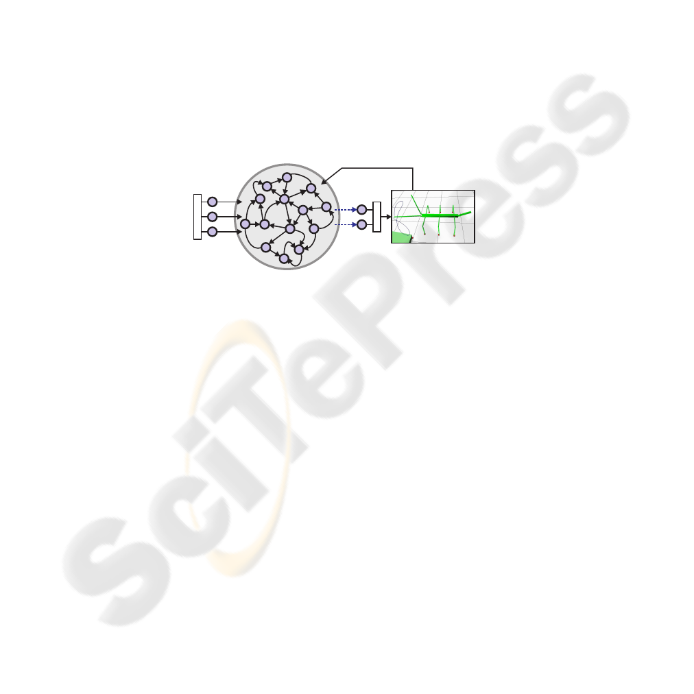
Fig.1. General structure of an echo state network. Solid arrows indicate ﬁxed, random connec-

tions, while dotted arrows are trainable readout connections. The output [????] sets the joint

angles of a bi-articular manipulator, e.g., an bio-inspired active tactile sensor. Joint angles are fed

back via the backprojection weight matrix W

back

2 Echo State Network

A basic, discrete-time ESN with a sigmoid activation functions was implemented in

Matlab

2009b. The purpose of this ESN was to control the joints of a bi-articular

manipulator that could serve as a bio-inspired, active tactile sensor. The overall goal

was to use the input to the ESN to set the tactile sampling pattern as desired. The state

update equations used are:

y(n) = W

out

x(n)

x(n + 1) = tanh(W

res

x(n) + W

u(n + 1) + W

back

y(n) + ν(n))

(1)

where u, x and y are the activations of the input, reservoir and output neurons, respec-

tively. ν(n) adds a small amount of uniformly distributed noise to the activation values

of the reservoir neurons. This tends to stabilize solutions, especially in models that use

output feedback for cyclic attractor learning [8]. W

, W

res

, W

out

and W

back

are

the input, reservoir, output and backprojection weight matrices. All matrices are sparse,

randomly initialised, and stay ﬁxed, except for W

out

. The weights of this linear output

layer are learned using ofﬂine batch training. During training, the teacher data is forced

into the network via the back-projection weights (teacher forcing), and internal reser-

voir activations are collected (state harvesting). After collecting internal states for all

training data, the output weights are directly calculated using ridge regression. Ridge

regression uses the Wiener-Hopf solution W

out

= R

−1

P and adds a regularization

term (Tikhonov regularization):

out

= (R + α

−1

P (2)

where α is a small number, I is the identity matrix, R = S

′

S is the correlation

matrix of the reservoir states and P = S

′

D is the cross-correlation matrix of the states

and the desired outputs. Ridge regression leads to more stable solutions and smaller

output weights, compared to ESN training using the Moore-Penrose pseudoinverse. A

value of α = 0.08 was used for all simulations in this paper.

3 Multi-objective Network Structure Optimization

Multi-objective optimization (MO) is a tool to explore trade-offs between conﬂicting

objectives. In the case of ESN optimization, the size of the reservoir versus the net-

work performance is the main trade-off. In MO, the concept of dominance replaces the

concept of a single optimal solution in traditional optimization. A solution dominates

another, if strictly one objective value is superior and all other objectives are at least

equal to the corresponding objective values of another solution. Following this deﬁni-

tion, multiple (possibly inﬁnite) non-dominated solutions can exist, instead of a single

optimal solution. The set of non-dominated or pareto-optimal solutions is called the

pareto front of the multi-objective problem. The goal of MO is to ﬁnd a good approx-

imation of the true pareto front, but usually MO algorithms converge to a local pareto

front due to complexity of the problem and computational constraints.

Usually, the structural parameters of an ESN are choosen manually by experience

and task demands. Here, the full set of free network parameters was optimized using

MO. The MO was performed with the function ’gamultiobj’ from the Matlab Genetic

Algorithm and Direct Search (GADS) Toolbox, that implements a variant of the ’Eli-

tist Non-dominated Sorting Genetic Algorithm version II’ (NSGA-II algorithm, [9]).

The network structure was encoded into the genotype as a seven-dimensional vector of

ﬂoating point numbers. The ﬁrst six structural parameters were the sparsity and weight

range of the input-, reservoir- and backprojection weights. The seventh parameter was

the number of reservoir neurons. The search range of the algorithm was constrained

to [0, 1] for the sparsity values, to [−5, 5] for the weight values and to [1, 100] for the

reservoir size ([1, 500] for the 4-pattern problem). The optimization was started with a

population size of 1000 and converged after around 120 generations. In each iteration of

the MO, all genomes were decoded into network structures, the networks were trained

and then simulated with random initial activations for 1000 frames per pattern. In order

to neglect the initial transient behaviour, the ﬁrst 50 iterations of network output were

rejected. The network output and the training patterns are usually not in-phase. The

best match between training pattern and network output was searched by phase-shifting

both output time courses by ± 50 frames relative to the training pattern and calculat-

ing the mean Manhattan distance across all pairs of data points. The training error was

then deﬁned as the smallest distance found in that range. The acceptable error threshold

(ﬁg.2) is expressed as the percentage of the amplitude of the training patterns, that is

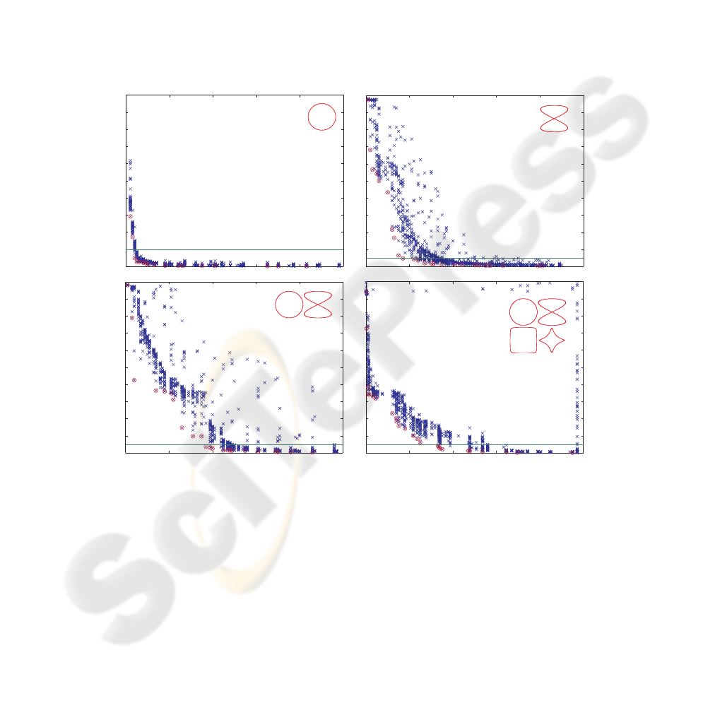
1.0 units for all patterns. The pareto front for a circular pattern (Fig.2a) reveals that

even very small networks are capable of learning and generating two sine waves with

identical frequency and 90 phase shift. The smallest network found had only 3 reservoir

neurons. Including the two output neurons, the overall network size was 5. In compar-

ison, 7 neurons are required for this task when using gradient-based learning methods

[10]. Network size increases with the complexity of the motor pattern, and especially

when having to store multiple patterns in a single network. Storing 4 patterns in a single

network required 166 reservoir neurons to reach an error below 5% (Fig.2d).

0 100 200 300 400 500

network size

0 20 40 60 80 100

network size

circle

eight

0 20 40 60 80 100

eight

0 20 40 60 80 100

0.005

0.01

0.015

0.02

0.025

0.03

0.035

0.04

0.045

0.05

error

circle

0.05

0.1

0.15

0.2

0.25

0.3

0.35

0.4

0.45

0.5

0.05

0.1

0.15

0.2

0.25

0.3

0.35

0.4

0.45

0.5

0.05

0.1

0.15

0.2

0.25

0.3

0.35

0.4

0.45

0.5

circle

eight

rectangle

star

error

a bb

Fig.2. Minimum reservoir size depends on task complexity. All panels show a set of pareto-

optimal solutions (red circles) and the ﬁnal population (blue crosses). (a) Learning a simple,

circular pattern. All networks with 3 or more neurons show an error below 1%. (b) Pareto-front

for the ﬁgure eight pattern. Learning this pattern requires a notably larger reservoir. Please note

the different scaling of the error compared to the easier circle task. Networks with 17 or more

neurons have an error below 5%. (c) Storing two motor patterns (circle and ﬁgure-eight) as cycli-

cal attractors in a single networkrequires 37 or more reservoir neurons for errors below 5%. (d)

Simultaneous learning of four patterns required 166 neurons.

4 Full Optimization of the Network Weights

From the pareto front of the two-pattern task, four candidate network structures were

selected and optimized further, using a single-objective genetic algorithm. This time,

all network weights except the output layer were fully optimized. The output layer was

still trained by ridge regression. An initial random population of 200 parents was cre-

ated from the network structure information of the selected candidate solutions with 4,

14, 26 and 37 reservoir neurons. Network weights were constrained to [−5, 5] and de-

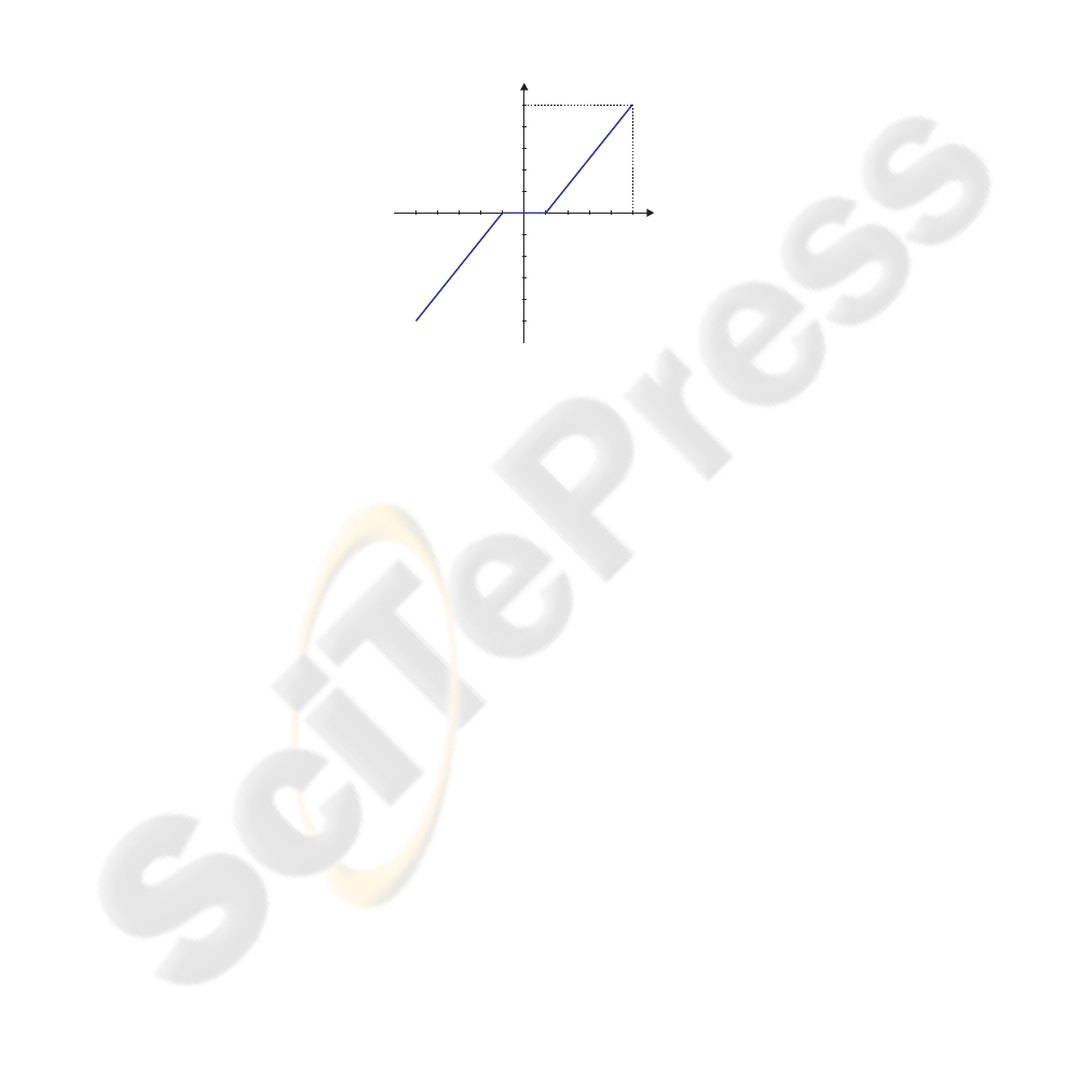
coded from the genome with a threshold function that preserves sparsity. The threshold

function sets a weight to zero, if the genome value is between -1 and 1, see ﬁg.3.

-1-5

-5

weight value

genome value

Fig.3. Threshold function that decodes genome values into weight values, preserving sparse

weight coding.

The Genetic Algorithm (GA) options were set to ranked roulette wheel selection,

20 elitist solutions, 80% crossover probability with scattered crossover and self adap-

tive mutation. Other options were left at their default values (see GADS toolbox, Mat-

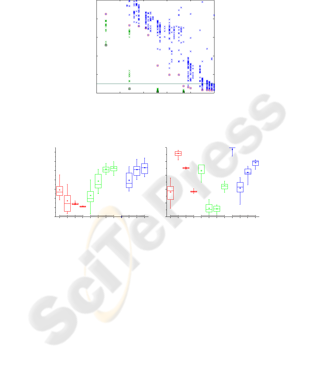
lab2009b). The GA-optimization was repeated 20 times for each network size. Fig.

4a shows the improvement in performance compared to the MO structure optimiza-

tion run. A small network with only 14 reservoir neurons could reproduce the learned

patterns with an error of 2.3%. Weight range and connectivity after optimization was

analysed with an unpaired Wilcoxon rank sum test. Signiﬁcant differences in connec-

tivity and weight range were found (Fig. 4b) with a clear trend for smaller reservoir

weights and less reservoir connectivity with increasing network sizes. Both input- and

backprojection weights tend to increase with reservoir size (Fig. 4a). Although standard

ESNs usually have full connectivity for input- and backprojectionweights, evolutionary

optimization seems to favor sparse connectivity for smaller networks, when given the

choice (Fig. 4b).

4.1 Hierarchical Evolutionary Optimization

In the previous section, individual solutions of the MO structural evolution were se-

lected and optimized further on the weight level, using a GA. Both steps can be com-

bined by performing a full-weight GA optimization for each iteration of the MO. This

20 30 40 50

network size

0.05

0.1

0.15

0.2

0.25

error

Fig.4. Subsequent full-weight matrix optimization improves performance. Additional optimiza-

tion of the four best networks of the two-pattern task with a reservoir size of 4, 14, 26 and 37

neurons. Starting from the best multi-objective solution, 20 GA runs were performed. a) Green

crosses indicate the best ﬁtness values of each run. Black squares indicate the overall best solu-

tions that were found.

0,0

0,2

0,4

0,6

0,8

1,0

1,2

1,4

4 14

0,0

0,2

0,4

0,6

0,8

1,0

connectivity

weight range

network size

* **

** ** **

** **** ** ** ** ** **

4 14

network size

Fig.5. Optimal weight range and connectivity depends on reservoir size. Network structure after

full-weight optimization of the selected networks from ﬁg.4. a) Weight range of all non-zero

weights of the reservoir (red), the backprojection weights (green) and the input weights (blue).

b) Connectivity (percentage of non-zero weights). Boxplots show 5%, 25%, 50%, 75% and 95%

quantiles of N=20 datapoints. * p ¡ 0.05; ** p ¡ 0.01.

way, the pareto front improves by moving closer towards the origin of both optimiza-

tion objectives. This nested, hierarchical optimization is computationally demanding.

To speed up the convergenceof the MO, good solutions of the full-weight GA are stored

in an archive, keeping each iteration of the MO accessible. In subsequent iterations, the

archived genome having the closest structure is injected into the new population of the

full-weight GA. Good networks can emerge faster by facilitating cross-over with the

archived solutions. This way, the full-weight optimization does not need to start from

scratch in each iteration. See Fig.6 for hierarchical optimization of the two-pattern task.

The MO had a population size of 200, running - at each iteration - a full-weight opti-

0 10 20 30 40 50

0.05

0.1

0.15

0.2

0.25

network size

error

0 10 20 30 40 50

0.05

0.1

0.15

0.2

0.25

network size

error

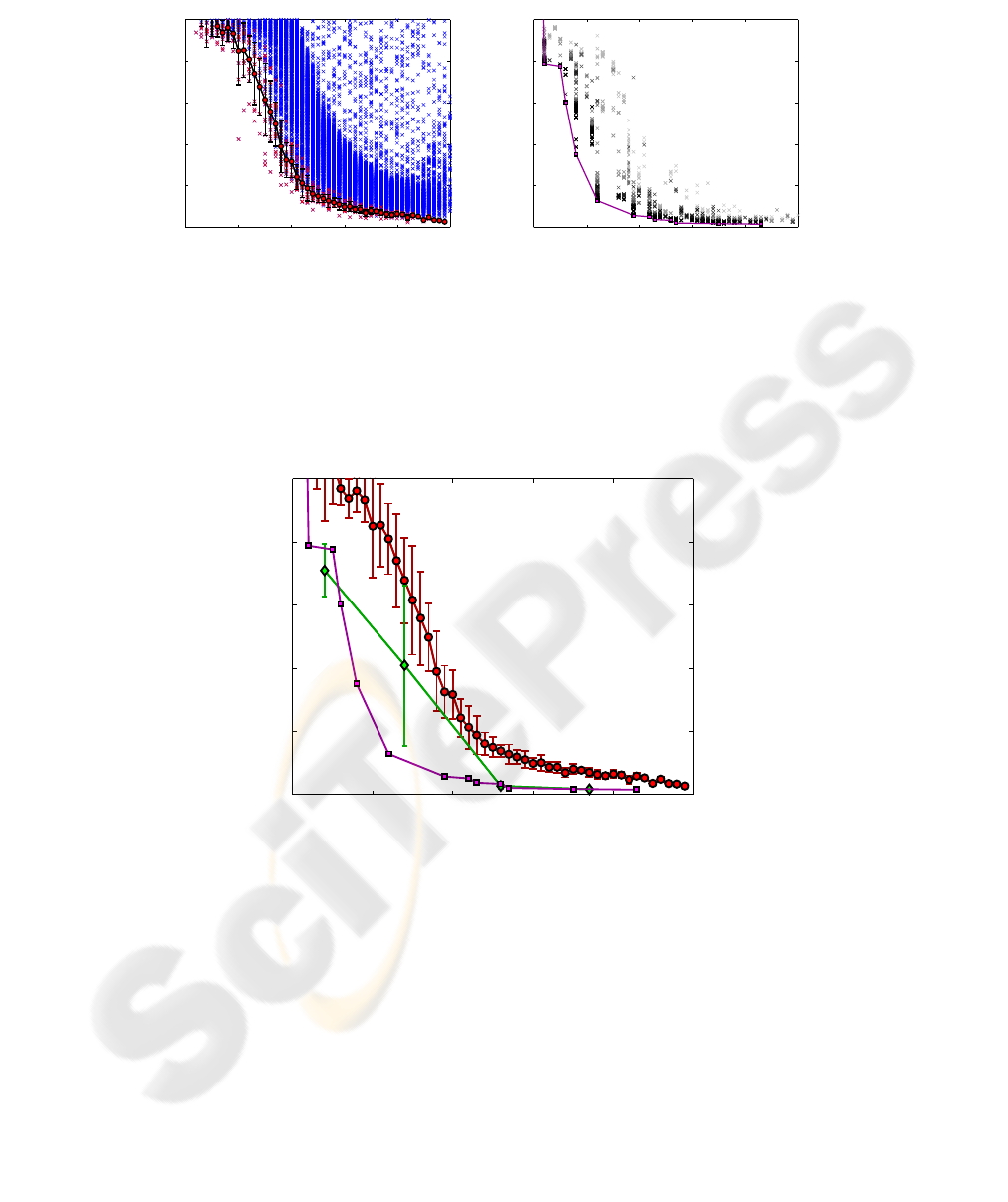
Fig.6. Left graph: Average pareto front from N=30 repetitions of the strucural MO. Blue crosses

show the ﬁnal populations, red crosses show the pareto fronts, and the red circles show the mean

and standard deviation of the pareto-optimal solutions for each network size. Right graph: Hier-

archically nesting a full-weight GA optimization into the MO optimization gives a more accurate

approximation of the true pareto front, as compared to structural MO alone. The plot shows a sin-

gle run of the nested MO-GA optimization over 25 generations. Crosses show the population at

each generation in grey levels ranging from light grey (ﬁrst generation) to black (last generation).

A single run outperforms the best solutions found in 30 runs of the structural MO, see Fig.7.

0 10 20 30 40 50

0.05

0.1

0.15

0.2

0.25

network size

error

0 10 20 30 40 50

0.05

0.1

0.15

0.2

0.25

network size

error

Fig.7. Comparison of the different optimization runs. The structural MO is shown in red (cir-

cles), full-weight optimization of selected solutions from the structural MO in green (diamonds),

and the hierarchical optimization in magenta (squares). A single run of the nested, hierarchical

optimization shows almost the same performance as the full-weight optimization from section 4.

mization with a population size of 20 individuals for 50 generations. Fig. 7 compares

the pareto fronts of the different optimization strategies. A single run of the nested op-

timization algorithm achieves almost the same result as the combination of structural

and subsequent full-weight optimization.

5 Dynamic Network Behaviour

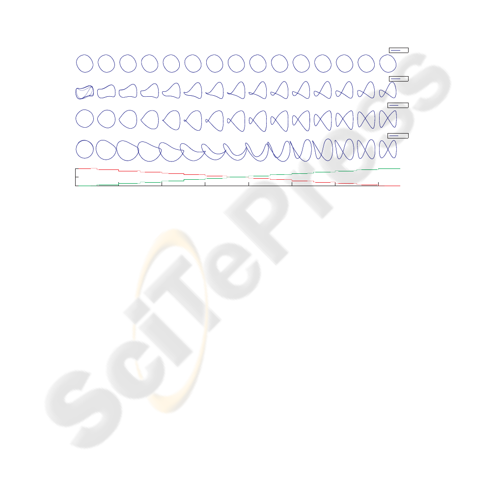
Most of the smaller networks show an unexpected behaviour. They are able to interpo-

late between the learned patterns, generating novel, not explicitly trained outputs. Fig.

8 shows the dynamical responses from the ﬁttest networks of section 4.1. The ﬁrst in-

put value was changed gradually in 15 steps from 1.0 to 0.0, while the second input

was changed from 0.0 to 1.0. A gradual morphing from the circular to the ﬁgure-eight

pattern can be observed. It is surprising, that already a small ESN with six reservoir neu-

rons can store two different patterns. Larger networks tend to converge to ﬁxed points

for input values other than the trained ones. This interpolation effect might be applied

to complex and smooth behaviour generation for neural network controlled robots.

N=2

N=6

N=12

N=33

0 2 4 6 8 10 12 14

0.5

Fig.8. Dynamic behaviour of selected networks with different reservoir sizes (blue trajectories).

Shifting the dynamics of the networks by gradually changing the ﬁrst input value (red) from 1.0

to 0.0 and the second input (green) from 0.0 to 1.0 in 15 steps. Changing the input to the network

causes a slow morphing between the two learned patterns, allowing to generate new patterns that

were not explicitly trained. Especially the small networks keep stable with no chaotic regions.

Larger networks tend to converge to ﬁxed points for input values other than zero or one.

6 Conclusions

Using MO, good candidate network structures can be selected as starting points for a

followup whole-network optimization and ﬁne-tuning using genetic algorithms. Both

steps can be combined into a nested, hierarchical multi-objective optimization. The re-

sulting pareto front helps to identify small and sufﬁciently efﬁcient networks that are

able to store multiple motor patterns in a single network. This distributed storage of

motor behaviours as attractor states in a single net is in contrast to earlier, local module

based approaches. ”If sequences contain similarities and overlap, however, a conﬂict

arises in such earlier models between generalization and segmentation, induced by

this separated modular structure.” [3]. By choosing a feasible model capacity, over-

ﬁtting and the risk of unwanted - possibly chaotic - attractor states is reduced. Also,

with the right choice of the network size, an interesting pattern interpolation effect can

be evoked. Instead of using a classic genetic algorithm for ﬁne-tuning of the network

weights, new, very fast and powerful black box optimisation algorithms [11] [12] could

further increase network performance and allow to ﬁnd even smaller networks for bet-

ter generalisation. ESNs can be used for direct control tasks ( see [13]) and scale well

with a high number of training patterns and motor outputs [14]. A more complex simu-

lation, for example of a humanoid robot, will show if direct, attractor-based storage of

parameterized motor patterns is ﬂexible enough for complex behaviour generation.

References

1. Tani, J., Itob, M., Sugitaa, Y.: Self-organization of distributedly represented multiple behav-

ior schemata in a mirror system: reviews of robot experiments using rnnpb. Neural Networks

17 (2004) 1273 – 1289

2. Haruno, M., Wolpert, D. M., Kawato, M.: Mosaic model for sensorimotor learning and

control. Neural Computation 13(10) (2001) 2201–2220

3. Yamashita, Y., Tani, J.: Emergence of functional hierarchy in a multiple timescale neural

network model: A humanoid robot experiment. PLoS Computational Biology 4 (11) (2008)

4. Werbos, P.: Backpropagation through time: what it does and how to do it. In: Proceedings

of the IEEE. Volume 78(10). (1990) 1550–1560

5. J¨ager, H., Haas, H.: Harnessing nonlinearity: Predicting chaotic systems and saving energy

in wireless communication. Science 304 (2004) 78 – 80

6. Jaeger, H.: Tutorial on training recurrent neural networks, covering bppt, rtrl, ekf and the

”‘echo state network”‘ approach. Technical Report GMD Report 159, German National

Research Center for Information Technology (2002)

7. Hochreiter, S., Bengio, Y., Frasconi, P., Schmidhuber, J.: Gradient ﬂow in recurrent nets: the

difﬁculty of learning long-term dependencies. In S. C. Kremer, J. F. K., ed.: A Field Guide

to Dynamical Recurrent Neural Networks. IEEE Press (2001)

8. Jaeger, H., Lukosevicius, M., Popovici, D., Siewert, U.: Optimization and applications of

echo state networks with leaky integrator neurons. Neural Networks 20(3) (2007) 335–352

9. Deb, K., Pratap, A., Agarwal, S., Meyarivan, T.: A fast and elitist multiobjective genetic

algorithm: Nsga-ii. IEEE Transactions on Evolutionary Computation 6, No. 2 (2002) 182–

197

10. Pearlmutter, B. A.: Learning state space trajectories in recurrent neural networks. Neural

Computation 1 (1989) 263–269

11. Kramer, O.: Fast blackbox optimization: Iterated local search and the strategy of powell. In:

The 2009 International Conference on Genetic and Evolutionary Methods (GEM’09). (2009)

in press.

12. Vrugt, J. A., Robinson, B. A., Hyman, J. M.: Self-adaptive multimethod search for global

optimization in real-parameter spaces. Evolutionary Computation, IEEE Transactions on

13(2) (2008) 243–259

13. Krause, A. F., Bl¨asing, B., D¨urr, V., Schack, T.: Direct Control of an Active Tactile Sen-

sor Using Echo State Networks. In: Human Centered Robot Systems. Cognition, Interac-

tion, Technology. Volume 6 of Cognitive Systems Monographs. Berlin Heidelberg: Springer-

Verlag (2009) 11–21

14. J¨ager, H.: Generating exponentially many periodic attractors with linearly growing echo

state networks. technical report 3, IUB (2006)