WHEELED-ROBOT NAVIGATION WITH VELOCITY

UPDATING ON ROUGH TERRAINS

Farid García and Matías Alvarado

Centro de Investigación y de Estudios Avanzados-IPN, Departamento de Computación

Av. Instituto Politécnico Nacional 2508, San Pedro Zacatenco, CP 07360, México DF, México

Keywords: Autonomous Navigation, Roughness Recognition, Velocity Updating, Wheeled-Robots.

Abstract: For navigation on outdoor surfaces, usually having different kind of roughness and soft irregularities, this

paper proposal is that a wheeled robot combines the gradient method for path planning, alongside it adjusts

velocity based on a multi-layer fuzzy neural network; the network integrates information about the

roughness and the soft slopes of the terrain to compute the navigation velocity. The implementation is

simple and computationally low-cost. The experimental tests show the advantage in the performance of the

robot by varying the velocity depending on the terrain features.

1 INTRODUCTION

Robotic autonomous navigation throughout outdoor

terrains is highly complex. Obstacle detection and

avoidance for no collision as well as the terrain

features information for no slides are both required.

Environment data must be quick and accurately

processed by the robot’s navigation systems for a

right displacing. Besides, when information from

human remote controllers is not quick available, the

autonomous robots should be equipped for

convenient reactions, particularly in front of

unpredicted circumstances. Actually, by moving on

outdoors, the autonomous robot’s velocity control

regarding the terrain features, beyond the obstacle

location and avoidance, it has been few attended and

it is a weakness for efficient and safe navigation

nowadays.

For wheeled-robots navigation on terrains, it is

necessary data about the surface features such that

automated safe navigation is ensured. The feature

which this work focuses is the surface roughness

where the robot moves on. The robot’s velocity

during real navigation depends on the terrain

roughness.

Outdoor autonomous robots are particularly

relevant employed for terrain exploration missions.

The terrain difficulties of soon system planets –like

Mars– to move through soil, rocks and slopes,

requires the usage of robots with the highest degree

of autonomy to overcome such difficulties. In Earth

exploration missions where human lives may be in

dangerous circumstances, the autonomous robots are

as well required. For instance, search of explosive

minas, active volcano craters exploration to

determine the eruption risk.

Kelly and Stentz (1998) propose a navigation

system for outdoors robots which includes

perception, mapping and obstacle avoidance.

Regarding the environment perception, Lambert et

al. (2008) introduces a probabilistic modelling useful

to avoid or to mitigate eventual collisions, which is

used for updating a robot braking action. Selekwa et

al. (2008) and Ward & Zelinsky (2000) addressed

the navigation and path planning of an autonomous

robot which varies the velocity according to the

proximity of obstacles detected by infrared sensors.

So far, all the referred works on outdoor

autonomous robots do not include in their proposals

information about terrain surface roughness during

navigation. In this work, two algorithms are

implemented for robot autonomous navigation, one

for path planning and the other for velocity updating

regarding the terrains features. The present proposal

is tested with a small wheeled-robot moving over

outdoors terrains containing grass, ground, garden

sand and soil, as the ones in

Figure 1 and Figure 2. It

is assumed that the robot can move on slopes with

inclination angles less than 15 degrees; otherwise,

the slopes are considered as obstacles, thus, the

robot wraps them, in order to overcome them.

277

Garc

ıa F. and Alvarado M. (2010).

WHEELED-ROBOT NAVIGATION WITH VELOCITY UPDATING ON ROUGH TERRAINS.

In Proceedings of the 7th International Conference on Informatics in Control, Automation and Robotics, pages 277-284

 SciTePress

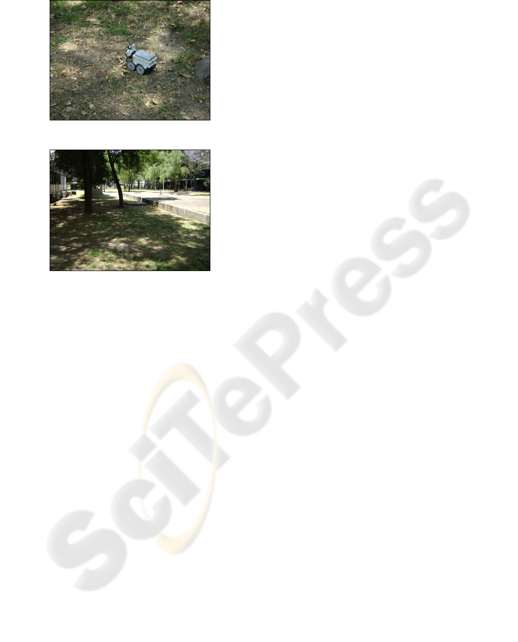
Figure 1: Robot’s navigation outdoor surface.

Figure 2: Test environment.

Surface textures are captured via artificial vision,

after image processing the estimation of the terrain

roughness as well as the slopes inclinations are

gotten. Then, the algorithms output indicates the

velocity the robot can achieve. Bright and uniform

lighting during navigation is required to guaranty

consistent roughness recognition; therefore the

presence of shadows, which treatment is a hard task

to pattern recognition (Kahraman and Stegmann,

2006), is out of the scope of this work.

During outdoors navigation, human drivers

estimate the convenient vehicle velocity by

regarding their previous experience when driving on

similar terrain textures. In other words, humans

estimate how rough, in average, the terrain is,

instead if specific texture details are recognized.

Human drivers that navigate on uneven terrains

do not need to know about specific details but on the

textures appearance average. The average

recognition of ranges of textures as the humans learn

is the behave experience to be mimicked and

implemented to strength the robots’ navigation

abilities. The algorithms for path planning differ

depending on the type of application, exploration on

unknown terrains (Seraji and Howard, 2002), car

navigation on roads (Sun et al., 2006), planet

exploration (Seraji and Werger, 2007) or indoor

navigation (Ward and Zelinsky, 2000), or if the

environment is either dynamic (Kim et al., 2007) or

static (Wang and Liu, 2005).

For our purpose, the robot moves on the

calculated path by adjusting its velocity depending

on the terrain features. The path planning algorithm

called gradient method, in static environments,

recalculates the path in real time whenever an

obstacle is found (Konolige, 2000). The gradient

method is integrated for our navigation proposal.

The rest of the article is organized as follows:

Section 2 summarizes the closest antecedents in the

field of autonomous navigation; then, the method

and architecture of the fuzzy neural network for

speed updating, together with the gradient method

for path planning are introduced. Section 3 describes

the integration of both algorithms for wheeled-robot

navigation, together with the tests and experimental

results. Discussion in Section 4, then the paper ends

with conclusions in Section 5.

2 VELOCITY UPDATING BY

FUZZY NEURAL NETWORK

2.1 Terrain Roughness Recognition

The classification of terrain roughness has almost no

received attention, and just recently is being a bit

more attended. For instance, Larson et al. (2005)

analysis the terrain roughness by means of spatial

discrimination which then is (meta-) classified.

Seraji and Howard (2002) assess the navigation

strategy with the terrain’s features of roughness,

slopes and discontinuity. Ishigami et al. (2007)

generate a path over a rough terrain with a terrain-

based criterion function, and then the robot is

controlled so as to move on the chosen path. In

Brooks and Iagnemma (2009) do roughness

recognition by using artificial vision, so recognition

of novel textures is later to off-line recognition

training from sample texture. Pereira et al. (2009)

plotted maps of terrains incorporating roughness

information that is based on the measurement of

vibrations occurring in the suspension of the vehicle;

this online method can recognize textures at the

moment the vehicle passes over them, what is a

limitation for velocity updating.

For velocity updating according to the terrain

features, our proposal sets to imitate as human

beings do. For safe navigation on irregular terrains,

the human’s velocity estimation is via imprecise but

enough surface texture recognition. When a human

driver notes a new texture, he uses his experience to

ICINCO 2010 - 7th International Conference on Informatics in Control, Automation and Robotics

278

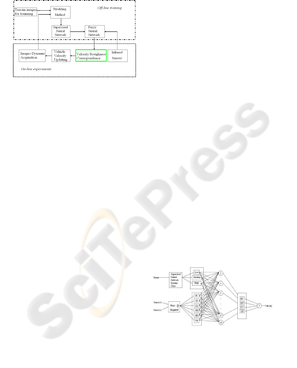
Figure 3: The proposal diagram.

estimate how rough the texture is, and then he

decides the car driving speed without slide risks.

As illustrated in the diagram of Figure 3, in the

first step, the terrain’s textures are neural-net-

clustered in a roughness meta-class: a Supervised

Neural Network (SNN) classifies textures forming

the meta-class; then, a Fuzzy Neural Network (FNN)

extends the supervised one, matches each terrain

roughness with the corresponding robot velocity

meanwhile the robot navigates safely.

Slopes are detected by two infrared sensors. One

infrared sensor is located in the frontal part of the

robot does parallel ray projection to the robot’s

motion; the other sensor projects its ray directly to

the floor perpendicular to the first sensor. The

inclination angle of slopes is computed by

trigonometric operations.

The off-line and on-line steps to adapt velocity

regarding the terrains roughness and the inclination

slopes while navigating are next described:

Roughness Identification (Off-line Training)

1) Select representative images of the terrain

textures, where the robot moves on.

2) Characterize the texture using the

Appearance Based Vision method which

computes the principal components of the

images distribution.

3) Train the SNN with the texture-roughness

relationship previously established by the

human expert driver.

4) Train the FNN to determine the velocity

regarding the texture roughness as well as the

inclination angle of slopes, according to an

expert driver’s directives, make the fuzzy sets

and the inferece IF-THEN rules system.

Velocity Updating and Robot’s Motion (On-line

Steps)

5) Acquisition of terrain images with the robot’s

camera.

6) The SNN classifies the texture and assigns its

roughness, this data is forwarded to the FNN.

7) The FNN inputs are both, the texture

roughness and the slope inclination angle (to

determine if the robot can pass on the slope,

or should move around it).

8) With the texture roughness and slope

inclination data, the FNN updates the

velocity. The robot’s mechanical control

system adjust the velocity.

9) The cycle is repeated as the robot moves, and

the velocity is cycle updated.

2.2 The Fuzzy Neural Network

This section introduces the five-layer fuzzy neural

network, whose output sets the velocity the robot

can achieve safely. The terrain features recognition

followed by the robot velocity tuning is shown in

Figure 4. The roughness and slope input data are

assessed and then used to adjust the robot’s velocity,

that is the FNN output data, see Table 1. The FNN

first layer inputs are the slope size and the texture

roughness, the second layer sets the terms of input

membership variables, the third sets the terms of the

rule base, the fourth sets the term of output

membership variables, and in the fifth one, the

output is the robot’s velocity. The textures

roughness is classified in three fuzzy sets, High (H),

Medium (M) and Low (L). The inclination angles of

slopes are classified in six fuzzy sets: Plain (Pl),

Slightly Plain (SP), Slightly Sloped (SS), Moderato

Sloped (MS), High Slope (HS) and Very High (VH).

The FNN output values are either: High Velocity

(HV), Moderate Velocity (MV), Low Velocity (LW)

or Stop (ST). Membership functions of the input and

output variables terms denote the corresponding

texture roughness, slope inclination and velocity,

respectively.

Figure 4: The Fuzzy Neural Network.

The fuzzy-making procedure maps the crisp

input values to the linguistic fuzzy terms with

membership values in [0,1]. In this work the

trapezoid membership functions (MF) for texture

WHEELED-ROBOT NAVIGATION WITH VELOCITY UPDATING ON ROUGH TERRAINS

279

variable and the triangle MF for angle variable are

respectively used. The FL inference rules governing

the input - output relationship are in the Table 1.

Taking X, Y, Z as variables of the respective

predicates, the form of inference rules is:

IF Slope angle is X AND Roughness is Y THEN

Velocity is Z.

The de-fuzzy procedure maps the fuzzy output

from the inference mechanism to a crisp signal.

When the robot finds a slope steeper than the

allowed threshold, it stops, and evaluates which

movement to make, whose decision concerns to path

planning. The gradient method (Konolige, 2000) is

integrated to present proposal.

2.3 The Gradient Method for Path

Planning

The gradient method requires a discrete

configuration of the navigation space in which the

path cost function is sampled. At each point of the

workspace, the gradient method uses a navigation

function to generate a gradient field that represents

the optimum path to the target point. The gradient of

navigation function indicates the path direction with

lowest cost, at each point in the navigation space;

this optimum path to the target is continuously

calculated, and is determined based on the length

and the proximity to obstacles, in addition to any

other criteria that may be chosen. By itself, the

gradient method can lead the path with the lowest

cost in static and completely unknown

environments; this method is efficient for real time

monitoring the movements of mobile robots

equipped with laser beams.

3 THE NAVIGATION

ALGORITHM

The robot autonomous navigation requires the

concurrent operation of path planning and velocity

estimation algorithms. The first step is to create a

virtual map of the robot navigation space; hence the

surface is divided into squares for providing the

required detail level of space model. The next step is

to calculate the optimal path between initial and goal

locations using the gradient method.

After path planning, the texture recognition

algorithm is turned on to determine the robot

velocity. The roughness surface data in addition to

information from sensors that measure the slopes

Table 1: The velocity updating fuzzy rules.

Rule

No.

Input Output

Slope angle Roughness Velocity

1 Pl L HV

2 Pl M HV

3 Pl H HV

4 SP L MV

5 SP M HV

6 SP H HV

7 SS L MV

8 SS M MV

9 SS H HV

10 MS L LV

11 MS M MV

12 MS H MV

13 HS L LV

14 HS M LV

15 HS H MV

16 VH L ST

17 VH M ST

18 VH H LV

inclination are processed. Hence, the robot receives

the instruction to move at the estimated velocity in

the prior determined trajectory. If during the trip the

sensors detect an obstacle or slopes with inclination

greater than 15 degrees, the robot stops and the

velocity estimation algorithm is turned off; the

obstacle is registered and a new path to the goal

location is recalculated. After that, the velocity

estimation algorithm is turned on again, and the

robot learns to move in the new trajectory at the

estimated speed. Otherwise, i.e., if the robot does not

find an obstacle on its path, then its speed is

updated.

Note that the velocity estimation algorithm is not

being executed all the time, but it is turned off when

the robot finds an obstacle; at this circumstance, the

camera records the obstacle images instead of

surface texture. If the velocity estimation algorithm

would not be turned off, the velocity would be

estimated based on images of the obstacle texture,

what is wrong; furthermore, in front of obstacle the

robot should overcomes the obstacle with specific

movements and the velocity change is irrelevant.

The robot stops when it determines that has

reached the goal location. The robot computes its

location from the distance it has travelled since the

initial location, by using odometry. The following

list summarizes the robot navigation steps, see

Figure 5:

1. Create a virtual map of robot space

navigation, surface discretization,

ICINCO 2010 - 7th International Conference on Informatics in Control, Automation and Robotics

280

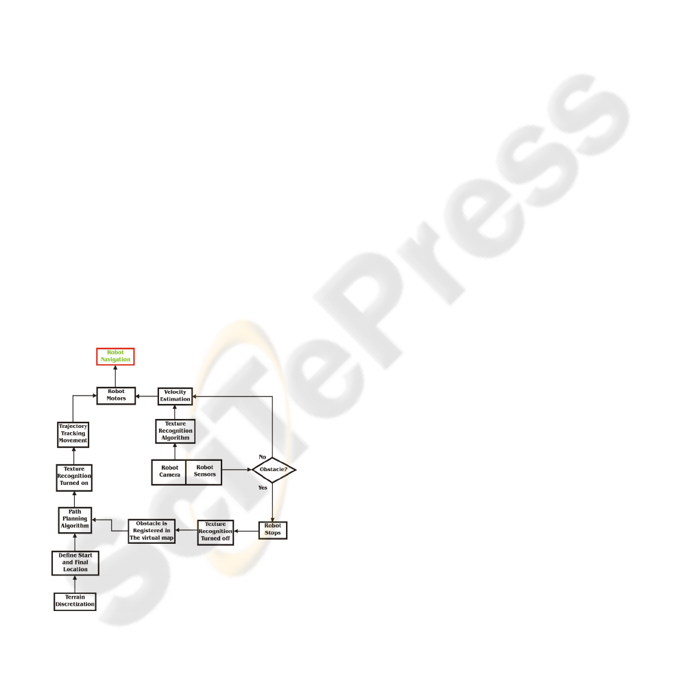
2. Define the initial and goal locations of the

robot,

3. Compute the path with the gradient method,

4. Artificial vision is turned on for texture

recognition,

5. Velocity is estimated with data from textures

and slopes of the surface,

6. The robot receives the order to advance along

the path at the estimated velocity,

7. The robot velocity is updated when a change

in texture is recognized, or if sensors detect a

slope on the surface, or if both events occur,

8. If sensors detect an obstacle, or if slope

inclination is greater than 15 degrees, then

the robot stops and texture recognition

algorithm is turned off, return to step 3;

Otherwise, velocity is updated, return to step

9. The robot stops when it has reached the goal

location or destination.

3.1 Experimental Step

A car-like rover from the Bioloid robot transformer

kit (ROBOTIS, 2010) is used, which uses a

processing unit, four servomotors for power

transmission to the wheels, two infrared sensors

located in the robot front, and a wireless camera on

top-front of the robot. The robot dimensions are 9.5

cm width per 15 cm length. In these experiments the

FNN is trained with terrain textures from images in

Figure 1.

Figure 5: Path Planning and Velocity estimation

algorithms running concurrently.

In this platform it is used a personal computer

(PC) and the processor of the robot, to form a

master-slave architecture, wirelessly communicated.

On the PC are implemented and executed the path

planning and velocity estimation algorithms. The

robot, on one hand, reports to the PC the sensors

readings and wirelessly transmits the images

captured by the camera. On the other hand, the robot

performs the movements in accordance with

instructions that the PC communicates it. The

experiments are performed in the environment

shown in

Figure 2, whose area is 2.25 m

, covered

with dust, soil, dry leaves, branches and 2 cm-high

grass; it contains rocks and small earth-mounds. The

goal point is located 2.12 meters in a straight line

from the initial location of the robot.

There were conducted 30 tests divided into three

parts, using the path planning algorithm. In first part,

the tests were performed at medium constant

velocity 6.95 cm/s; in the second part at the

maximum velocity the robot can reach 13.88 cm/s.

The other tests were performed with velocity

updating, combining path planning and velocity

updating algorithms. Table 2 shows the results.

With velocity updating, both the detection of the

robot environment and path planning are

strengthened. By adjusting the velocity according to

surface characteristics, safety increases and/or the

travel time of the robot decreases. That is, if it

detects that the surface is slippery then the robot

slows down, although the robot spends more time to

reach the goal location, the probability that the robot

has an accident decreases.

3.2 Results and Navigation

Performance

The common standards criterion to evaluate the

performance of robots is (Dai et al., 2007), (Matthies

et al., 1995): accurate estimation of the robot

location, fast and accurate detection of the robot

environment and reliable path planning for moving

from one place to another without colliding with

obstacles in unknown environments. This is true for

this proposal and adds the following:

• The total time it takes the robot to make the

route and,

• Comparing the distance travelled by the robot

with the straight line distance between the

initial and goal locations.

When the robot moves at medium constant

velocity (6.94 cm/s), it runs 107.72% of the straight

line distance between the initial and goal locations.

The travel distance is increased because of the

obstacle avoidance and the location estimation errors

WHEELED-ROBOT NAVIGATION WITH VELOCITY UPDATING ON ROUGH TERRAINS

281

Table 2: Autonomous navigation results with and without

velocity updating.

Constant velocity

With

velocity

updating

Navigation

velocity

6.94 cm/s

13.88

cm/s

8.65 cm/s

(average

velocity)

Navigation

distance

228.5 cm

111.29

220.33 cm

Navigation

time

43.10 s 19.08 s 32.55 s

generated by the slippage of wheels. On the other

hand, when the robot moves at maximum constant

velocity (13.88 cm/s) runs, on average, 52.46% of

the path. The plausible explanation is that when the

robot moves at maximum velocity the wheels slip

more often and therefore the location estimation of

the robot becomes very imprecise. With velocity

updating the robot travels the 103.86% of the

straight line distance between the initial and goal

locations. In this case the distance is less than with

medium constant velocity because the wheel

slippage is less frequent, see Table 3. By updating

the velocity the robot moves slower in areas that

favour the slippage of wheels, for instance loose

soil. Because of there are fewer slippages, the

location estimation of the robot is more accurate and

consequently the robot approaches the goal location.

The navigation time with velocity updating is

32.41% less and 41.38% higher than medium and

maximum constant velocity, respectively. It is noted

that with medium constant velocity the robot travels

a path with good accuracy but spends more time

doing the travelling. With maximum constant

velocity the travelling is fast but the accuracy to

traverse the path is very bad. With velocity updating

performance is improved because the precision of

the robot in the travelling of the trajectory is good

and is performed in less time, i.e., the robot moves at

optimum velocity, depending on surface

characteristics, avoiding wheel slippage. With our

approach the average velocity represents 62.13% of

the maximum velocity the robot can reach.

4 DISCUSSION

Within the present approach, the robot moves on

surfaces with different kinds of textures, to make

navigation more versatile than such related works.

The Martian surface can be considered as a special

case of our approach because these surfaces are

Table 3: Percentage of travelled distances, with maximum

and medium constant velocity; and with velocity updating.

Constant Velocity With

velocity

updating

Medium Maximum

Percentage

of distance

travelled

107.72% 52.46% 103.86%

covered with sand and rocks, i.e., there is only one

type of roughness. Actually, for the purpose of

autonomous navigation on rough terrains is not a

requisite to recognize textures at a high detail level.

The high precision methods on details recognition

are not the adequate but failed for supporting robots

navigation –strongly some times. In addition, the

detailed recognition of surfaces is computationally

expensive, but a low consume of resources is

recommended through autonomous navigation.

Our approach can be improved on the location

estimation of the robot. So far, it has been used

odometry only to calculate the robot location. Most

of the works, if not all, that employ odometry use

other tools to estimate the location of the robot such

as electronic compasses (Seraji and Werger, 2007),

sonar sensors (Dai et al., 2007), GPS (Matthies et

al., 1995), among others. However, velocity

updating reduces wheel slippage and the drift errors

are small or occur less often.

On the other hand, the proposed algorithms are

not limited to be applied to small vehicles. They can

be extrapolated to other vehicles, depending on the

particular characteristics, which define the

appropriate rules of the vehicle operation. The

algorithm is scalable to different vehicles by using

as parameters their particular characteristics, such as

weight, size and motor power, tires material and tire

tread, among others.

In this proposal we claim that for velocity

updating the experience of human drivers is

mimicking by using the inference system of the

fuzzy neural network, which model the operation of

the vehicle based on the driver experience.

There are works that model the vehicles driving

with differential equations (Nakamura et al., 2007),

(Kim et al., 2008), (Ward and Iagnemma, 2008). But

this approach is difficult because, in general,

differential equations are nonlinear, and their

solution is hard to obtain.

Within the algorithms testing, we have simulated

the path of a truck. These tests consisted of placing a

camera on the roof of the truck. The truck runs on

various types of textures. During the truck trips, the

camera recorded from a similar driver’s visual field

ICINCO 2010 - 7th International Conference on Informatics in Control, Automation and Robotics

282

the crossed surfaces. Then, texture images are

extracted from video recordings, which are

processed by the algorithms.

The velocity updating results are encouraging.

To process the 480×640-pixel images with the

microprocessor Centrino Core 2 Duo at 2 GHz and

1.99 Gb RAM, the algorithms time spent is small,

0.3 seconds. It leads to conclude that vehicles with

these computer capacities have enough time to react

or to break on the next 5 meters, as soon as they are

moving at 60 km/hr, which is a car maximum

velocity in the city, and a standard speed on

principal roads.

5 CONCLUSIONS

In this paper a proposal for wheeled robot navigation

on outdoor surfaces with different kind of roughness

and soft irregularities is presented. The robot

integrates the path planning gradient method with a

multi-layer fuzzy neural network in order to adjust

velocity, by regarding the roughness and the slopes

of the terrain. The artificial vision implementation is

computationally low-cost. Wheeled-robot navigation

becomes more efficient and safe because of the

velocity updating. That is because, whenever the

robots navigates, the velocity is updated by

regarding the terrains characteristics, the wheel

slippage is significant reduced, hence improving, the

precision to achieve the goal location as well as the

navigation time; thereafter, the risk that the robot

suffers an accident is also decreased. On the

opposite, without velocity updating it becomes more

difficult the goal location approach as reported

results show.

ACKNOWLEDGEMENTS

The authors would like to thank the financial support

of CINVESTAV-IPN, Centro de Investigación y de

Estudios Avanzados del Instituto Politécnico

Nacional. As well Farid García, scholarship no.

207029, would like to thank the financial support of

CONACyT, Consejo Nacional de Ciencia y

Tecnología.

REFERENCES

Brooks, C.A. and Iagnemma, K. (2009). Visual Detection

of Novel Terrain via Two-Class Classification. In:

Proceedings of the 2009 ACM Symposium on Applied

Computing, 1145-1150.

Dai, X., Zhang, H. and Shi, Y. (2007). Autonomous

Navigation for Wheeled Mobile Robots-A Survey. In:

Second International Conference on Innovative

Computing, Information and Control, September 5-7,

Kumamoto, Japan, 2207-2210.

Ishigami, G., Nagatani, K. and Yoshida, K. (2007). Path

Planning for Planetary Exploration Rovers and Its

Evaluation Based on Wheel Slip Dynamics. In: IEEE

International Conference on Robotics and

Automation, April 10-14, Roma, Italy, 2361-2366.

Kahraman, F. and Stegmann, M.B. (2006). Towards

Illumination-Invariant Localization of Faces Using

Active Appearance Models. In: 7th Nordic Signal

Processing Symposium, June 7-9, Rejkjavik, Iceland,

Kelly, A. and Stentz, A. (1998). Rough Terrain

Autonomous Mobility – Part 2: An Active Vision,

Predictive Control Approach. Autonomous Robots,

5(2), 163-198.

Kim, P.G., Park, C.G., Jong, Y.H., Yun, J.H., Mo, E.J.,

Kim, C.S., Jie, M.S., Hwang, S.C. and Lee, K.W.

(2007). Obstacle Avoidance of a Mobile Robot Using

Vision System and Ultrasonic Sensor. In: Third

International Conference on Intelligent Computing,

August 21-24, Qingdao, China, 545-453.

Kim, Y.C., Min, K.D., Yun, K.H., Byun, Y.S. and Mok,

J.K. (2008). Steering Control for Lateral Guidance for

an All Wheel Steered Vehicle. In: International

Conference on Control, Automation and Systems.

October 14-17, Seoul, Korea, 24-28.

Konolige, K. (2000). A Gradient Method for Realtime

Robot Control. In: Proceedings of the IEEE/RSJ

International Conference on Intelligent Robots and

Systems. October 31 – November 5, Takamatsu, Japan,

639-646.

Lambert, A., Gruyer, D., Pierre, G.S. and Ndjeng, A.N.

(2008). Collision Probability Assessment for Speed

Control. In: 11

International IEEE Conference on

Intelligent Transportation Systems. October 12-15,

Beijing, China, 1043-1048.

Larson, A.C., Voyles, R.M. and Demir, G.K. (2005).

Terrain Classification Using Weakly-Structured

Vehicle/Terrain Interaction. Autonomous Robots,

19(1), 41-52.

Nakamura, S., Faragalli, M., Mizukami, N., Nakatani, I.,

Kunii, Y. And Kubota, T. (2007). Wheeled Robot with

Movable Center of Mass for Traversing over Rough

Terrain. In: Proceedings of the IEEE/RSJ

International Conference on Intelligent Robots and

Systems. October 29 – November 2, 1228-1233.

Matthies, L., Gat, E., Harrison, R., Wilcox, B., Volpe, R.

and Litwin, T. (1995). Mars Microrover Navigation:

Performance Evaluation and Enhancement.

Autonomous Robots, 2(4), 291-311.

Pereira, G.A.S., Pimenta, L.C.A., Chaimowicz, L.,

Fonseca, A.F., de Almeida, D.S.C., Correa, L.Q.,

Mesquita, R.C. and Campos, F.M. (2009). Robot

Navigation in Multi-Terrain Outdoor Environments.

WHEELED-ROBOT NAVIGATION WITH VELOCITY UPDATING ON ROUGH TERRAINS

283

International Journal of Robotic Research, 28(6), 685-

700.

ROBOTIS Co., (2010). http://www.robotis.com.

Selekwa, M.F., Dunlap, D.D., Shi, D. and Collins, E.G.

(2008). Robot Navigation in Very Cluttered

Environments by Preference-Based Fuzzy Behaviors.

Robotics and Autonomous Systems, 53(3), 231-246.

Seraji, H. and Howard, A. (2002). Behavior-Based Robot

Navigation on Challenging Terrain: A Fuzzy Logic

Approach. IEEE Transactions on Robotics and

Automation, 18(3), 308-321.

Seraji, H. and Werger, B. (2007). Theory and Experiments

in SmartNav Rover Navigation. Autonomous Robots,

22(2), 165-182.

Sun, Z., Bebis, G. and Miller, R. (2006). On-Road Vehicle

Detection: A Review. IEEE Transaction on Pattern

Analysis and Machine Intelligence, 28(5), 694-711.

Wang, M. and Liu, J.N.K. (2005). Behavior-Blind Goal-

Oriented Robot Navigation by Fuzzy Logic. In:

Proceedings of Knowledge-Based Intelligent

Information and Engineering Systems, 686-692.

Ward, C.C. and Iagnemma, K. (2008). A Dynamic-Model-

Based Wheel Slip Detector for Mobile Robots on

Outdoor Terrain. IEEE Transactions on Robotics,

24(4), 821-831.

Ward, K. and Zelinsky, A. (2000). Acquiring Mobile

Robot Behaviors by Learning Trajectory Velocities.

Autonomous Robots, 9(2), 113-133.

ICINCO 2010 - 7th International Conference on Informatics in Control, Automation and Robotics

284