MINING TIMED SEQUENCES WITH TOM4L FRAMEWORK

Nabil Benayadi and Marc Le Goc

LSIS Laboratory, University Saint Jerome, Marseille, France

Keywords:

Sequential patterns, Information-theory, Temporal knowledge Discovering, Chronicles models, Markov pro-

cesses.

Abstract:

We introduce the problem of mining sequential patterns in large database of sequences using a Stochastic

Approach. An example of patterns we are interested in is : 50% of cases of engine stops in the car are

happened between 0 and 2 minutes after observing a lack of the gas in the engine, produced between 0 and

1 minutes after the fuel tank is empty. We call this patterns “signatures”. Previous research have considered

some equivalent patterns, but such work have three mains problems : (1) the sensibility of their algorithms with

the value of their parameters, (2) too large number of discovered patterns, and (3) their discovered patterns

consider only ”after“ relation (succession in time) and omit temporal constraints between elements in patterns.

To address this issue, we present TOM4L process (Timed Observations Mining for Learning process) which

uses a stochastic representation of a given set of sequences on which an inductive reasoning coupled with an

abductive reasoning is applied to reduce the space search. The results obtained with an application on very

complex real world system are also presented to show the operational character of the TOM4L process.

1 INTRODUCTION

The aim of Timed Data Mining techniques is to dis-

cover temporal knowledge from a set of timed mes-

sages sequences.

The general context is given in the Figure 1: a dy-

namic process is monitored with a Monitoring Cog-

nitive Agent (MCA) that writes timed messages in a

database. The dynamic process can be a manufac-

turing process, a telecommunication network or web

servers for example. The timed messages are con-

cerned with alarms or warnings, or with the starting

or the stopping of tasks. The ”learning process” aims

at discovering the temporal knowledge that character-

ize the behavior of the monitored dynamic process to

improve its management. This problematic is nowa-

days crucial in most of the industrial and the service

sectors.

In this paper, we introduce the problems of min-

ing such a pattern : 50% of cases of engine stops in

the car are happened between 0 and 2 minutes after

observing a lack of the gas in the engine, produced

between 0 and 1 minutes after the fuel tank is empty.

We call this patterns “signatures”. Finding signatures

are valuable in many ﬁelds, for example, when target-

ing markets using DM (Direct Mail), market analysts

can use signatures to learn what actions they should

take and when they should act to inform their cus-

tomers to buy. In the industrial domain, operators can

use signatures to control and supervise the process

variables before maintaining the process in an equilib-

rium state. Other applications include predicting dis-

ease, forecasting weather, if we ﬁnd signature : 60%

of storms go through area B between 1 and 3 days

after they strike area A, we can take steps to cope a

disaster in the area B. We propose in this paper the ba-

sis of the TOM4L process (Timed Observations Min-

ing for Learning process) deﬁned to discover signa-

tures among timed messages in large database of se-

quences. TOM4L process avoids also the two remains

problems of Timed Data Mining techniques: the sen-

sibility of the Timed Data Mining algorithms with the

value of their parameters and the too large number of

generated patterns. TOM4L avoids these two prob-

lems with the use of a stochastic representation of a

given set of sequences on which an inductive reason-

ing coupled with an abductive reasoning is applied to

reduce the space search. The next section recalls the

basis of the main Timed Data Mining techniques and

presents a (very) simple illustrative example to show

the main problems of previous approaches. Next, sec-

tion 3 introduces the basis of the TOM4L process and

the section 4 describes the results obtained with an

application of the TOM4L process on very complex

111

Benayadi N. and Le Goc M. (2010).

MINING TIMED SEQUENCES WITH TOM4L FRAMEWORK.

In Proceedings of the 12th International Conference on Enterprise Information Systems - Artiﬁcial Intelligence and Decision Support Systems, pages

111-120

DOI: 10.5220/0002958401110120

 SciTePress

Figure 1: Temporal knowledge discovery context.

real world system monitored with a large scale knowl-

edge based system, the Sachem system of the Arcelor-

Mittal Steel group. The section 5 makes a synthesis

of the paper and introduces our current works.

2 RELATED WORKS

Discovering temporal knowledge from the timed mes-

sages is a problem that can be studied from multi-

ple points of view and a lot of scientiﬁc domains

are concerned with this problem, speciﬁcally Ma-

chine Learning and Data Mining (cf. (Roddick and

Spiliopoulou, 2002) for a complete state of the art).

The Timed Data Mining approachesaims at avoid-

ing this problem. The basic principle consists in using

a representativeness criteria, typically the support of a

sequential pattern, to build the minimal set of sequen-

tial patterns that describes the given set of sequences.

The support s(p

) of a pattern p

is the number of se-

quences in the set of sequences where the pattern p

is observed. A frequent pattern is a pattern p

with

a support s(p

) greater than a user deﬁned thresholds

s(p

) ≥ S. A frequent pattern is interpreted as a reg-

ularity or a condensed representation of the given set

of sequences.

The Timed Data Mining techniques differs de-

pending on whether the initial set of sequences is a

singleton or not. The second case is the simpler be-

cause the decision criteria based on the support is di-

rectly applicable to a set of sequences. One of the ﬁrst

application can be found in the market basket analysis

(Agrawal and Psaila, 1995) with the AprioriAll algo-

rithm that has been improved with the SPAM (Ayres

et al., 2002) or the SPADE (Zaki, 2001) algorithms.

When the initial set of sequences contains a

unique sequence, the notion of windows has been in-

troduced to deﬁne an adapted notion of support. The

ﬁrst way consists in deﬁning a ﬁxed size of windows

that an algorithm like Winepi (Mannila et al., 1995)

shifts along the sequence: the sequence becomes then

a set of equal length sub-sequences and the support

s(p

) of a pattern can be computed (Vilalta and Ma,

2002; Weiss and Hirsh, 1998). The second way con-

sists in building a window for an a priori given pattern

. With the Minepi algorithm for example (Mannila

and Toivonen, 1996), a window W = [t

[ is a min-

imal occurrence of p

if p

occurs in W and not in

any sub-window of W. In practice, a maximal win-

dow size parameter maxwin must be deﬁned to bound

the search space of patterns. A similar approach is

proposed in (Dousson and Duong, 1999) to discover

chronicle models, an abstract representation of pat-

terns.

The Timed Data Mining approaches presents two

main problems. The ﬁrst is that the algorithms require

the setting of a set of parameters: the discovered pat-

terns depends therefore of the tuning of the algorithms

(Mannila, 2002). The second problem is the number

of generated patterns that is not linear with threshold

value S of the decision criteria s(p

) ≥ S. In prac-

tice, to obtain an interesting set of frequent pattern,

S must be small, and the number of frequent is huge

((Han and Kamber, 2006)). But generally, only a very

small fraction of the discovered patterns are interest-

ing. This leads to use interestingness measures to

build a minimal set of frequent patterns having some

potential to be signiﬁcative. The mostly used interest-

ingness measures are based on the Information the-

ory (Shannon, 1949) like the j-measure (Smyth and

Goodman, 1992) and the mutual information (Cover

and Thomas, 1991). Let us take a simple example to

illustrate these two basic problems of the Timed Data

Mining approaches.

The illustrativeexample is a simple dynamic SISO

system y(t) = F · x(t) where F is a convolution opera-

tor. This example is used trough this paper to illustrate

the claims.

Let us deﬁning two thresholds

and

for the

input variable x(t) and the output variable y(t). These

two thresholds respectively deﬁnes two ranges for

each of the variables: rx

=] − ∞,

], rx

, +∞],

=] − ∞,

] and ry

, +∞]). Let us suppose

that there exists a (very simple) program that writes

a constant when a signal enter in a range. Such

a program writes the constant 1 (resp. H) when

x(t) (resp. y(t)) enters in the range rx

(resp. ry

)

and 0 (resp. L) when x(t) (resp. y(t)) enters in

the range rx

(resp. ry

). The evolution of the

x(t) in the ﬁgure 2 leads to the following sequence:

= {(1, t

), (H,t

), (0, t

), (L,t

), (1, t

), (H, t

(0,t

), (L,t

), (1,t

), (H, t

), (0,t

), (L,t

), (1,t

(H, t

), (0, t

), (L,t

), (1, t

), (H, t

), (0, t

(L,t

), (1,t

), (H,t

), (0,t

), (L,t

)}.

To illustrate the sensibility of the Winepi and the

Minepi algorithms with the parameters, we deﬁnes

two sets of parameters and apply the algorithms to the

sequence

. In the ﬁrst set of parameters, the window

ICEIS 2010 - 12th International Conference on Enterprise Information Systems

112

x(t)

y(t)

1 3 5 7 9 11 13 15 17 19 21 23

2 4 5 8 10 12 14 16 18 20 22 24



Figure 2: Temporal evolution of variables x and y.

width w and window movement v for Winepi are both

set to 4 (this is the ideal tuning) and for Minepi, the

max window is set to 4 and the minimal frequency is

ﬁxed to 6 (this is also the ideal tuning). In the sec-

ond set of parameters, the window width and window

movement of Winepi are equal to 8 and the support

is equal to 3. The minimal frequency for Minepi is

set to 8. The table 1 provides the number of patterns

discovered by each algorithm with the two sets of pa-

rameters.

These two experimentations show the sensibility

of the Winepi and the Minepi algorithms with the pa-

rameters: from the ﬁrst set to the second, the number

of patterns increase of more than 626% for Winepi,

and more than 18666% from Minepi. The main prob-

lem is the too large number of discovered patterns.

The paradox is then the following: to ﬁnd the ideal set

of parameters that minimizes the number of discov-

ered patterns, the user must know the system while

this is precisely the global aim of the Data Mining

techniques. There is then a crucial need for another

type of approach that is able to provide a good solu-

tion for such a simple system and provide operational

solutions for real world systems. The aim of this pa-

per is to propose such an approach: the TOM4L pro-

cess (i.e. Timed Observation Mining for Learning)

which ﬁnd only 4 relations with the example without

any parameters.

Table 1: Number of discovered patterns.

Winepi Minepi

First parameter set 15 15

Second parameter set 94 2800

3 FINDING SIGNATURES

The TOM4L process is based on the Theory of Timed

Observations of (Le Goc, 2006) that deﬁnes an in-

ductive reasoning and an abductive reasoning on a

stochastic representation of a set of sequences Ω =

{

}, this set being or not a singleton.

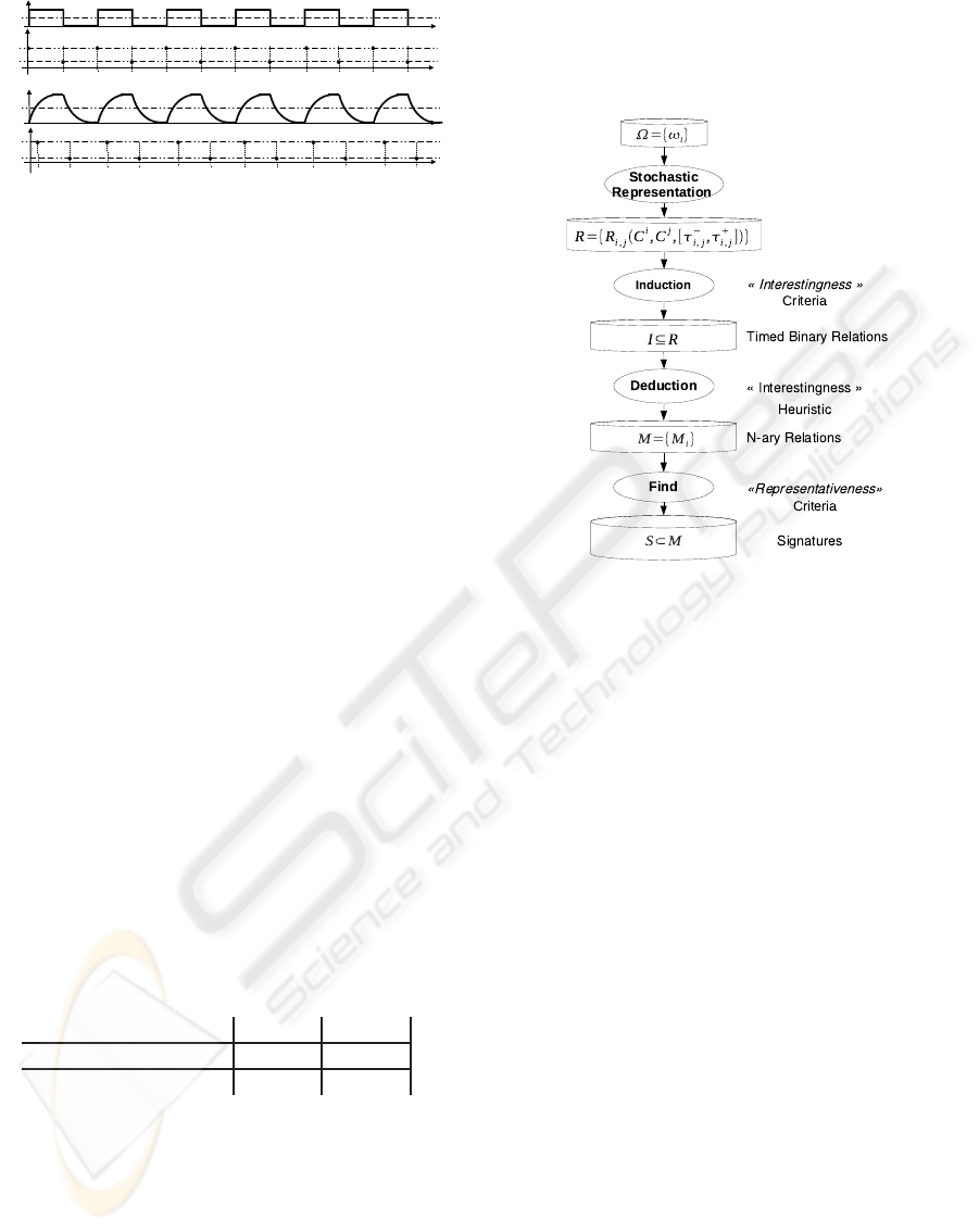
This theory provides the mathematical foundations of

the four steps Timed Data Mining process of Figure

3 that reverses the usual Data Mining process in or-

der to minimize the size of the set of the discovered

patterns:

Figure 3: The four steps of TOM4L approch.

1. Stochastic Representation of a set of sequences

Ω = {

}. This step produces a set of timed bi-

nary relations of the form R

i, j

, [

−

i, j

]).

2. Induction of a minimal set of timed binary rela-

tions. This step uses an interestingness criteria

based on the BJ-measure describes in the follow-

ing section.

3. Deduction of a minimal set of n-ary relations.

This step uses an abductive reasoning to build a

set of n-ary relations that have some interest ac-

cording to a particular problem.

4. Find the minimal set of n-ary relations being rep-

resentatives according to the problem. This step

corresponds to the usual search step of sequential

patterns in a set of sequences in Minepi or Winepi.

The discovered n-ary relations discovered in the last

step are called signatures. The next section provides

the basic deﬁnitions of the Timed Observations The-

ory.

3.1 Basic Deﬁnitions

A discrete event e

is a couple (x

) where x

the name of a variable and

is a constant. The

constant

denotes an abstract value that can be as-

signed to the variable x

. The illustrative example al-

lows the deﬁnition of a set E of four discrete events:

E = {e

≡ (x, 1), e

≡ (x, 0), e

≡ (y, H), e

≡ (y, L)}.

MINING TIMED SEQUENCES WITH TOM4L FRAMEWORK

113

A discrete event class C

= {e

} is an arbitrary set of

discrete event e

= (x

). Generally, and this will be

true in the suite of the paper, the discrete event classes

are deﬁned as singletons because when the constants

are independent, two discrete event classes C

{(x

)} and C

= {(x

)} are only linked with the

variables x

and x

((Le Goc, 2006)). The illustrative

example allows the deﬁnition of a set Cl of 4 discrete

event classes: Cl = {C

= {e

}, C

= {e

}, C

= {e

}}.

An occurrence o(k) of a discrete eventclassC

= {e

= (x

), is a triple (x

) where t

is the time

of the occurrence. An occurrence o(k) ≡ (x

)

is called a timed observation in (Le Goc, 2006) be-

cause it can always be interpreted as the assignation

of the abstract value

to the variable x at time t

(i.e. o(k) ⇔ x(t

) =

). The idea is that a timed ob-

servation is supposed to be written by a program that

implements the following speciﬁcation:

∃t

k−1

∈ ℜ, t

k−1

< t

k−1

) ≤

∧ x

) >

⇒ o(k) ≡ (x

)

(1)

When useful, the rewriting rule o(k) ≡ (x

) ≡

(k) will be used in the following.

A sequence Ω = {o(k)}

k=1...n

, is an ordered set

of n occurrences C

(k) ≡ (x

). The illustra-

tive example deﬁnes the following sequence: Ω =

{(C

(1), C

(2), C

(3), C

(4), C

(5), C

(6), C

(7),

(8), C

(9), C

(10), C

(11), C

(12), C

(13), C

(14),

(15), C

(16), C

(17), C

(18), C

(19), C

(20), C

(21),

(22), C

(23), C

(24)}. As a consequence, a se-

quence Ω = {o(k)}

k=1...n

deﬁnes:

• A set K = {k}, k ∈ ℵ, of time index.

• A set Γ = {t

}, t

∈ ℜ of times generated by a

continuous clock structure (t

k−2

− t

k−1

6= t

k−1

−

• A set ∆ = {

} of constants.

• A set X = {x

} of variables.

• A set E = {e

} of discrete event e

= (x

) de-

ﬁned on X × ∆.

• A set Cl = {C

} of discrete event classes (also

called timed observation classes).

Le Goc (Le Goc, 2006) shows that when the con-

stants

∈ ∆ are independent, a sequence Ω = {o(k)}

deﬁning a set Cl = {C

} of m classes is the superposi-

tion of m sequences

= {C

(k)}:

Ω = {o(k)} =

[

i=1...m

= {C

(k)} (2)

The Ω sequence of the illustrative example is then

the superposition of four sequences

= {C

(k)}:

= {C

(1),C

(5),C

(9),C

(13),C

(17),C

(21)}

= {C

(3),C

(7),C

(11),C

(15),C

(19),C

(23)}

= {C

(4),C

(8),C

(12),C

(16),C

(20),C

(24)}

= {C

(2),C

(6),C

(10),C

(14),C

(18),C

(22)}

3.2 Stochastic Representation

The stochastic representation transforms a set of

sequences

= { o(k)} in a Markov chain X =

(X(t

);k > 0) where the state space Q = {q

}, i =

1. . . m, of X is confused with the set of m classes

Cl = {C

} of Ω =

[

Consequently, two successive occurrences (C

(k− 1),

(k)) correspondto a state transition in X: X(t

k−1

) =

−→ X(t

) = q

. The conditional probability

P[X(t

) = q

|X(t

k−1

) = q

] of the transition from a

state q

to a state q

in X corresponds then to the

conditional probability P



(k) ∈ Ω|C

(k− 1) ∈ Ω



of observing an occurrence of the class C

at time t

knowing that an occurrence of a class C

at time t

k−1

has been observed:

∀i, j, ∀k ∈ K,

P[X(t

) = q

|X(t

k−1

) = q

] = P



(k) ∈ Ω|C

(k− 1) ∈ Ω



≡ p

∑

l,l6=i

The transition probability matrix P = [p

i, j

] of X

is computed from the contingency table N = [n

i, j

where n

i, j

∈ N is the number of couples (C

(k),C

(k+

1)) in Ω. The table 2 is the contingency table N of the

sequence Ω of the illustrative example.

Table 2: Contingency table N = [n

i, j

] of Ω.

Total

0 0 6 0 6

0 0 0 6 6

0 6 0 0 6

5 0 0 0 5

Total 5 6 6 6 23

The stochastic representation of a given set

Ω of sequences is then the deﬁnition of a set

R = {R

i, j

, [

−

])} where each the condi-

tional probability p

i, j

= P



(k) ∈ Ω|C

(k− 1) ∈ Ω



of each binary relation R

i, j

, [

−

]) is

not null. The timed constrains [

−

] is pro-

vided by a function of the set D of delays

D = {d

} = {(t

− t

)} computed from the bi-

nary superposition of the sequences

i, j

∪

−

= f

−

(D),

= f

(D). For example, the au-

thors of (Bouch´e, 2005) use the properties of the

Poisson law to compute the timed constraints:

−

= 0,

i, j

where

i, j

is the Poisson rate (i.e.

ICEIS 2010 - 12th International Conference on Enterprise Information Systems

114

the exponential intensity) of the exponential law that

is the average delay d

moy

∑

)

Card(D)

. But more

frequently, a min-max approach is used (Dousson and

Duong, 1999) :

−

= min(D

= max(D

The set R of the illustrative example is the

following: R = {R

1,H

, [

−

1,H

]),

0,L

, [

−

0,L

]), R

H,0

, [

−

H,0

]),

L,1

, [

−

L,1

])}.

3.3 Discrete Binary Memoryless

Channel Model

Considering a binary relation R

i, j

, [

−

]), a

sequence Ω deﬁning the set Cl of m classes with n

occurrences contains n − 1 couples (o(k), o(k + 1)).

Each of them is one of the four following types:

(k),C

(k + 1)), (C

(k),C

(k + 1)), (C

(k),C

(k +

1)), and (C

(k),C

(k + 1)), where C

(resp. C

) is an

abstract class denoting any classes of Cl but C

(resp.

The n−1 couples (o(k), o(k+ 1)) can then be seen as

n− 1 realizations of one of the four relations linking

two abstract binary variables X and Y of a discrete bi-

nary memoryless channel in a communication system

according to the information theory (Shannon, 1949),

where X(t

) ∈ {C

} and Y(t

k+1

) ∈ {C

} (Fig-

ure 4).

Figure 4: Two abstract binary variables connected by a dis-

crete memoryless channel.

To use this model, the number of occurrences of

the abstract classes C

and C

can not be the number

of the occurrences of the classes Cl −C

and Cl −C

but an average value:

• n

i, j

is the number of couples (C

(k),C

(k+ 1)) in

Ω.

• n

i, j

is the average number of couples

(k),C

(k+ 1)) in Ω:

• n

i, j

m− 1

∑

∀C

∈C

i,l

• n

i, j

is the average number of couples

(k),C

(k+ 1)) in Ω:

• n

i, j

m− 1

∑

∀C

∈C

l, j

• n

i, j

is the average number of couples

(k),C

(k+ 1)) in Ω:

• n

i, j

(m− 1)

∑

∀C

∈C

,∀C

∈C

l, f

This leads to m·(m− 1) binary contingency tables

of the form of the Table 3.

Table 3: Contingency table for X and Y.

∑

i, j

∑

y∈{ j, j}

i,y

i, j

∑

y∈{ j, j}

i,y

∑

x∈{i,i}

x, j

∑

x∈{i,i}

x, j

N =

∑

x∈{i,i},y∈{ j, j}

x,y

These contingency tables allow computing

two conditional probabilities matrix P

(i.e.

P(Y(t

k+1

)|X(t

))) and P

(i.e. P(X(t

)|Y(t

k+1

))(Table

4). These two matrix allow the deﬁnition of the BJ-

measure to build a criteria to evaluate the interest of a

binary relation R

i, j

, [

−

]).

Table 4: P

and P

matrix.

p(C

) =

i, j

p(C

) =

i, j

p(C

) =

i, j

p(C

) =

i, j

p(C

) =

i, j

p(C

) =

i, j

p(C

) =

i, j

p(C

) =

i, j

3.4 Evaluating the Interestingness of

Binary Relations

The idea for deﬁning an efﬁcient interestingness crite-

ria to induce binary relations is that if knowing C

(k)

increases the probability of observing C

(k + 1) (i.e.

p(C

) > p(C

)), then the observation C

(k) pro-

vides some information about an observation C

(k +

1) (Blachman, 1968).

We propose then to use the distance of Kullback-

Leibler D(p(Y|X = C

)kp(Y)) to evaluate the relation

between the a priori distribution p(C

) of an observa-

tion C

(k) and the conditional distribution p(C

MINING TIMED SEQUENCES WITH TOM4L FRAMEWORK

115

D(p(Y|X = C

)kp(Y)) =

p(Y = C

|X = C

) ×log



p(Y=C

|X=C

)

p(Y=C

)



p(Y = C

|X = C

) ×log



p(Y=C

|X=C

)

p(Y=C

)



(3)

One of the property of this distance is that

D(p(Y|X = C

)kp(Y)) = 0 when p(Y = C

|X = C

) =

p(Y = C

). This property means that when the distri-

butions p(Y = C

) and p(X = C

) are independent, the

Kullback-Leibler distance is null. This allows to de-

compose the Kullback-Leibler distance in two terms.

Deﬁnition 1. The BJL-measure BJL(C

) of binary

relation R(C

) is the right part of the Kullback-

Leibler distance D(p(Y|X = C

)kp(Y)):

• p(Y = C

|X = C

) < p(Y = C

) ⇒ BJL(C

) =

• p(Y = C

|X = C

) ≥ p(Y = C

) ⇒ BJL(C

) =

D(p(Y|X = C

)kp(Y))

Considering the discrete memoryless binary chan-

nel (Figure 4), the BJL(C

) is not null when

the observation C

(k) provides some information

about the observation C

(k). Symmetrically, when

BJL(C

) = 0, the observationC

(k) provides some

information about any observations but C

(k), that is

to say about an observation C

(k). This leads to de-

ﬁne the BJL-measure BJL(C

) of a binary relation

R(C

Deﬁnition 2. The BJL-measure BJL(C

) of a bi-

nary relation R(C

) is the left part of the Kullback-

Leibler distance D(p(Y|X = C

)kp(Y)):

• p(Y = C

|X = C

) < p(Y = C

) ⇒ BJL(C

) =

D(p(Y|X = C

)kp(Y))

• p(Y = C

|X = C

) ≥ p(Y = C

) ⇒ BJL(C

) =

This leads to the decomposition of the Kullback-

Leibler distance property:

D(p(Y|C

)kp(Y)) = BJL(C

) + BJL(C

) (4)

Looking at the Figure 4, the deﬁnition of the BJL-

measure decomposes the information provided by the

assignation X(t

) = C

(i.e. an observation C

(k)) be-

tween the assignation Y(t

k+1

) = C

(i.e. the obser-

vation C

(k + 1)) and the assignation Y(t

k+1

) = C

(i.e. the observation C

(k + 1)). In other words, the

BJL-measure evaluates the information distribution

between the next successor (C

(k + 1) or C

(k + 1))

of an observation C

(k) at time t

. The same rea-

soning can be done when considering the information

distribution between the predecessors X(t

) = C

X(t

) = C

of the assignation Y(t

k+1

) = C

Deﬁnition 3. The BJW-measure BJW(C

) of

binary relation R(C

) is the right part of the

Kullback-Leibler distance D(p(X|Y = C

)kp(X)):

• p(X = C

|Y = C

) < p(X = C

) ⇒ BJW(C

) =

• p(X = C

|Y = C

) ≥ p(X = C

) ⇒ BJW(C

) =

D(p(X|Y = C

)kp(X))

Symmetrically:

Deﬁnition 4. The BJW-measure BJW(C

) of bi-

nary relation R(C

) is the left part of the Kullback-

Leibler distance D(p(X|Y = C

)kp(X)):

• p(X = C

|Y = C

) < p(X = C

) ⇒ BJW(C

) =

D(p(X|Y = C

)kp(X))

• p(X = C

|Y = C

) ≥ p(X = C

) ⇒ BJW(C

) =

Again, the BJW-measure decomposes the

Kullback-Leibler distance D(p(X|Y = C

)kp(X)) in

two terms:

D(p(X|Y = C

)kp(X)) = BJW(C

)+BJW(C

)

The BJW-measure evaluates then the information

distribution between the predecessors (C

(k) orC

(k))

of an observation C

(k+ 1) at time t

k+1

The BJL-measure evaluates the information that

ﬂows in two successor relations of a discrete memo-

ryless binary channel (i.e. from X(t

) = C

to Y(t

k+1

Figure 4) and the BJW-measure evaluates the infor-

mation that ﬂows in two predecessor relations (i.e.

from X(t

) to Y(t

k+1

) = C

). Because (p(C

) <

p(C

)) ⇔ p(C

) < p(C

)), these two measures are

null at the same independence point. The information

ﬂowing trough these four relations can then be com-

bined in a single measure called the BJM-measure.

Deﬁnition 5. The BJM-measure BJM(C

) of a

binary relation R(C

) is the norm of the vector





BJL(C

)

BJW(C

)





• (p(C

) ≥ p(C

)) ∨ (p(C

) ≥ p(C

)) ⇒

BJM(C

) =

BJL(C

)

+ BJW(C

)

• (p(C

) < p(C

)) ∨ (p(C

) < p(C

)) ⇒

BJM(C

) = −

BJL(C

)

+ BJW(C

)

The minus sign is used to build a monotonous

measure that distinguishes the position of a relation

R(C

) around the independence point. The BJM-

measure BJM(C

) of a relation R(C

) is then

simply:

BJM(C

) =

BJL(C

)

+ BJW(C

)

(5)

−

BJL(C

)

+ BJW(C

)

ICEIS 2010 - 12th International Conference on Enterprise Information Systems

116

The maximum value BJM(C

)

max

(obtained

when n

i, j

= min(n

, n j)) and the minimum value of

BJM(C

)

min

(obtained when n

i, j

= 0) depend on

the ratio

i, j

. The comparison of two BJM-

measures is not possible. To avoid this problem, the

BJM-measure BJM(C

) is made linear with a M-

measure M(C

) deﬁned as follows:

Deﬁnition 6.

M(C

) =











BJM(C

)

BJM(C

)

max

if p(C

) > p(C

)

−

BJM(C

)

BJM(C

)

min

else

Whatever is the ratio

i, j

, the M-measure M(C

)

as the following properties:

• M(C

) = 1 ⇔ BJM(C

) = BJM(C

)

max

(ideal crisscross)

• M(C

) = 0, 5 ⇔ BJM(C

) = 0 (C

and C

are independent)

• M(C

) = 0 ⇔ BJM(C

) = BJM(C

)

min

and C

are not linked)

For example, the values of the M-measure

of the set R = {R

1,H

, [

−

1,H

]),

0,L

, [

−

0,L

]), R

H,0

, [

−

H,0

]),

L,1

, [

−

L,1

])} of the illustrative example

are given in table 5. This table shows that all the

relations of R are ideally mixed.

Table 5: Matrix M.

0 0 1 0

0 0 0 1

0 1 0 0

1 0 0 0

3.5 Inducing Binary Relations

In this example, the relations

1,H

, [

−

1,H

]) and R

0,L

, [

−

0,L

])

have not the same meaning than the relations

H,0

, [

−

H,0

]) R

L,1

, [

−

L,1

]):

only the two ﬁrst are linked with the system

y(t) = Fx(t), the two latter being only sequential

relation (i.e. the system computes the values of y(t),

not the values of x(t)).

To distinguish between these two kind of rela-

tions, the idea is to add noise in the initial set of

sequences. To this aim, we deﬁned the ”noisy” ob-

servation class C

err

the occurrences of which are

Table 6: The M values evolution with different

err

R(C

) R(C

)

0 1 1 1 1

6 0.75 0.56 1 0.63

12 0.78 0 1 0

18 0.61 0 0.79 0

24 0.55 0 0.55 0

30 0 0 0 0

randomly timed. If a relation R

i, j

, [

−

i, j

])

is a property of the system, then the time interval

between the occurrences of the C

and C

classes

will be more regular than if this relation is a purely

sequential relation. The table 6 shows the val-

ues of the M-measures of the relations R(C

R(C

), R(C

) and R(C

) with different

rate

err

− t

of noisy occurrences added in

Ω. For example, the sequence

with

err

= 18 is

the following:

= {C

(1), C

(2), C

err

(3), C

(4),

err

(5), C

(6), C

err

(7), C

err

(8), C

err

(9), C

(10),

(11), C

(12), C

(13), C

(14), C

err

(15), C

(16),

err

(17), C

(18), C

(19), C

err

(20), C

(21), C

(22),

err

(23),C

(24),C

(25),C

err

(26),C

(27),C

err

(28),

(29), C

err

(30), C

(31), C

(32), C

err

(33), C

(34),

err

(35), C

(36), C

err

(37), C

err

(38), C

err

(39),

(40), C

(41), C

err

(42)}. The table 6 shows that

when

err

∈ {12, 24}, the binary relations R(C

)

and R(C

) disappears. Naturally, when the noise

is too strong (

err

= 30), all the relations disappear:

this means that at least one occurrence C

err

(k) is sys-

tematically inserted between two occurrences of the

initial sequence Ω.

This example leads also to an operational prop-

erty of the M-measure: when

i, j

≫ 1 or

i, j

≪ 1,

one class plays the same role of a noisy class for the

other. This situation arises in the two following cases:

• n

i, j

≥ n

i, j

⇒ p(C

) ≥ 0.5. TheC

plays the role

of a noisy class for the class C

• n

i, j

≥ n

i, j

⇒ p(C

) ≥ 0.5. TheC

plays the role

of a noisy class for the class C

These two conditions are both evaluated when com-

paring the product p(C

) · p(C

) with

when p(C

) · p(C

) ≤

, M(C

) ≤ 0.5 and

the relation R

i, j

) can not be justiﬁed with the

M-measure. Inversely, when p(C

)· p(C

) >

M(C

) > 0.5 and the relation R

i, j

) has some

interest from the point of view of the M-measure.

MINING TIMED SEQUENCES WITH TOM4L FRAMEWORK

117

This leads to the following simple inducing rule that

uses the M-measure as interestingness criteria:

M(C

) > 0.5 ⇒ R

i, j

) ∈ I (6)

3.6 Deduction of N-ary Relations

The set I of binary relations contains then the minimal

subset of R where each relation R

i, j

) presents a

potential interest. From this set, the M-measure can

be used to build n-ary relations having some poten-

tial to be observed in the initial set Ω of sequences.

To this aim, the M-measure is used in an heuristic

h(m

i,n

) that guides an abductive reasoning to build

a minimal set M = {m

k,n

} of n-ary relations of the

form m

k,n

= {R

i,i+1

i+1

)}, i = k, ··· , n − 1, that

is to say paths leading to a particular ﬁnal observation

class C

. The heuristic h(m

i,n

) makes a compromise

between the generality and the quality of a path m

i,n

h(m

i,n

) = card(m

i,n

) × BJL(m

i,n

) × P(m

i,n

) (7)

In this equation, card(m

i,n

) is the number of relations

in m

i,n

, BJL(m

i,n

) is the sum of the BJL-measures

BJL(C

k−1

) of each relation R

k−1,k

k−1

) in

i,n

and P(m

i,n

) is the product of the probabilities as-

sociated with each relation in m

i,n

• BJL(m

i,n

) =

∑

k=card(m

i,n

),···,1

BJL



R(C

k−1

)



• P(m

i,n

) =

∏

i=card(m

i,n

),···,1

p(C

k−1

)

P(m

i,n

) corresponds to the Chapmann-

Kolmogorov probability of a path in the transition

matrix P = [p(k − 1, k)] of the Stochastic Represen-

tation. The interestingness heuristic h(m

i,n

) being

of the form

· ln(

), it can be used to build all the

paths m

i,n

where h(m

i,n

) is maximum (Benayadi and

Le Goc, 2008). For the illustrative example, the

deduction step found a set M of two binary relations

(M = I)

3.7 Find Representativeness N-ary

Relations

Given a set M = {m

k,n

)} of paths m

k,n

i,i+1

i+1

)}, i = k, ··· , n − 1, the TOM4L

process uses two representativeness criterion to build

the subset S ⊆ M containing the only paths m

k,n

being representative according the initial set Ω of

sequences. These criterion are a timed version of

support and conﬁdence notions:

Deﬁnition 7. Anticipation Rate.

The anticipation rate Ta(m

i,n

) of a n-ary relation m

i,n

No paths containing more than one binary relation can

be deduced from I.

is the ratio between the number of instances of m

i,n

Ω with the number of occurrences of the m

i,n−1

(i.e.

the n-ary relation m

i,n

without the last binary relation

n−1,n

n−1

)).

Deﬁnition 8. Cover Rate.

The cover rate Tc(m

i,n

) of a n-ary relation m

i,n

is the

ratio between the number of occurrences of m

i,n

with

the number of occurrences of the ﬁnal class C

of the

n-ary relation m

i,n

The anticipation rate Ta(m

i,n

) and the cover rate

Tc(m

i,n

) are criterion that allow to deﬁne an interest-

ingness criteria to ﬁnd interesting n-ary relations m

i,n

that are called ”Signatures”:

Deﬁnition 9. Signature.

An n-ary relation m

i,n

is a signature if and only if

Tc(m

i,n

) ≥ C and Ta(m

i,n

) ≥ A, where C ∈ [0, 1] ⊂ ℜ

and A ∈ [0, 1] ⊂ ℜ.

Given a set of sequences (typically Ω) and the

values of A and C, the ”BJT4S” algorithm computes

all the anticipation rate Ta(m

i,n

) and the cover rate

Tc(m

i,n

) of each sub-paths m

k,n

, k ≥ i, of each paths

i,n

of M to build the set S of signatures that sat-

isfy the conditions Tc(m

k,n

) ≥ C and Ta(m

k,n

) ≥ A.

To this aim, the ”BJT4S” algorithm represents the

sub-paths m

k,n

in DEVS models and uses an abstract

chronicle recognition engine to compute the corre-

sponding anticipation rate Ta(m

k,n

) and the cover rate

Tc(m

k,n

) (Le Goc et al., 2006). The complexity of

this algorithm is proportional with the number of sub-

paths and the size of the sequence so the smallest the

set M = {m

k,n

)} is (i.e. the most efﬁcient the inter-

estingness heuristic h(m

i,n

) is) , the faster the exe-

cution of the BJT4S algorithm is. For example, the

values of the cover rate and the anticipation rate of

both binary relations of M of the illustrative example

are 100%. So, S = M, S = {R

1,H

, [

−

1,H

]),

0,L

, [

−

0,L

])}. These signatures are the only

relations (patterns) that are linked with the system

y(t) = Fx(t). Comparing with the set of patterns

found by Apriori-like approaches, we can conﬁrm

from this illustrative example that TOM4L approach

converges towards a minimal set of operational re-

lations, which describe the dynamic of the process.

In the next section, we present the application of

TOM4L on a sequence generated by a very complex

dynamic process, blast furnace process. Due to the

process complexity, we can conﬁrm, without expe-

rience, that Apriori-like approaches fail to mine this

sequence.

ICEIS 2010 - 12th International Conference on Enterprise Information Systems

118

4 APPLICATION

Sachem is the name of the very large scale

knowledge-based system the Arcelor-Mittal Steel

group has developed at the end the 20th century to

help the operators to monitor, diagnose and control

the blast furnace, a very complex production process

(Le Goc, 2006).

With a Sachem system, the blast furnace behav-

ior is described with a series of occurrences of phe-

nomenon classes that corresponds to the observation

classes of TOM4L. The application is concerned with

the omega variable that reveals the management qual-

ity of the whole blast furnace. The omega is a very ab-

stract variable corresponding to the ratio of the num-

ber of carbon atoms used to produce a ton of hot

metal with the number of iron (f

) atoms it contains

(the studied blast furnace produces 6,000 tons of hot

metal per day). The values of omega are provided

by a mathematical model which is a set of 17 differ-

ential equations linking together 53 high level vari-

ables synthesizing the whole the blast furnace behav-

ior. This model is used to compute the ideal value

of omega corresponding to a perfectly adjusted blast

furnace: any distance from this ideal value means

that the blast furnace is not well managed. In a set

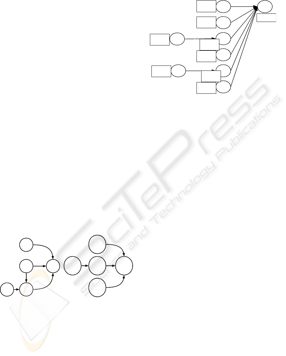
of expertise documents of 1995, the experts deﬁnes

the variable modiﬁcations that cause the main mod-

iﬁcations of omega (Figure 5, a): the top gas speed

(TGS), the ﬂame temperature (TF), the burden per-

meability (BD) and the size of the sinter (SS) through

the burden permeability. The studied sequence comes

Omega

1463, 1464

1465, 1467

TGS

1454, 1454

T°F

1217, 1216

1717, 1718

1719, 1719

1720,1721

1256,1257,1258

1259,1260,1262

1267,1269,1271

Omega

TGS

T°F

Figure 5: Expert’s (1995, a) and discovered relations (2009,

b).

from a blast furnace of Fos-Sur-Mer (France) from

08/01/2001 to 31/12/2001. It contains 7682 occur-

rences of 45 classes. For the 1463 class linked to

the omega variable, the search space contains about

= 3, 200, 000 binary relations. The inductive and

the abductive reasoning steps of TOM4L produces

a minimal set M of only 166 binary relations from

which the set S of signatures of ﬁgure 6 have been

discovered (Ta = 50% and Tc = 10%). The set S is

made with 50 binary relations.

14631454

1467

1217

[0,35h51m6s]

[0,142h15m22s

]

[0,57h6m248s]

1717

1464

[0,132h25m30s]

1267

[0,82h2m20s]

1718

[0,92h0m0s]

1465

[0,47h40m50s]

[0,110h24m0s]

Tc= 74 %

Ta=62 %

Tc=67%

Ta=164 %

Tc=14 %

Ta=62 %

Tc=19 %

Ta=328%

Tc= 22 %

Ta=100 %

Tc=29 %

Ta=156 %

Tc=53%

Ta=58 %

Tc= 71 %

Ta=138 %

Tc=98%

Figure 6: 1463 class signatures.

When substituting a class with its associated vari-

able (the omega variable with the class 1464 for ex-

ample) and the signatures of Figure 6 becomes the

graph (b) of Figure 5 that contains the graph of the

Expert’s in 1995. The only difference is the direction

of the relation between the variables TF and BD. This

result shows that when pruning the branches bring-

ing few information from a class to another, the BJ-

measure allows to consider only the branches with a

strong potentiality to be a signature: every signature

Figure 6 have a strong credibility according to the

laws governing the blast furnace. It is to note that the

same result is observed on the Apache system, a clone

of Sachem design to monitor and diagnose a galva-

nization bathe. As with the simple illustrative exam-

ple of this paper, this result shows that the TOM4L

process converges through a minimal set of binary

relations with the elimination of the non interesting

relations, despite of the complexity of the monitored

process.

5 CONCLUSIONS

This paper presents the basis of the TOM4L process

for discovering temporal knowledge from timed mes-

sages generated by monitored dynamic process. The

TOM4L process is based on four steps: (1) a stochas-

tic representation of a given set of sequences from

which is induced (2) a minimal set of timed binary

relations, and an abductive reasoning (3) is then used

to build a minimal set of n-ary relations that is used to

ﬁnd (4) the most representativen-ary relations accord-

ing to the given set of sequences. The induction and

the abductive reasoning are based on an interesting-

ness measure of the timed binary relations, that allows

eliminating the relations having no meaning accord-

ing to the given set of sequences. The results obtained

MINING TIMED SEQUENCES WITH TOM4L FRAMEWORK

119

with an application on a very complex real world pro-

cess (a blast furnace) are presented to show the opera-

tional character of the TOM4L process. These results

provide new insights about the blast furnace behavior.

So our current works are now focusing on the deﬁni-

tion of a verity principle that is required to qualiﬁed

the discovered relations.

REFERENCES

Agrawal, R. and Psaila, G. (1995). Active data mining.

In Fayyad, Usama, M. and Uthurusamy, R., editors,

First International Conference on Knowledge Discov-

ery and Data Mining (KDD-95), pages 3–8, Montreal,

Quebec, Canada. AAAI Press, Menlo Park, CA, USA.

Ayres, J., Flannick, J., Gehrke, J., and Yiu, T. (2002). Se-

quential pattern mining using a bitmap representation.

KDD02: Proceedings of the eighth ACM SIGKDD in-

ternational conference on Knowledge discovery and

data mining, pages 429–435.

Benayadi, N. and Le Goc, M. (2008). Using a measure

of the crisscross of series of timed observations to

discover timed knowledge. Proceedings of the 19th

International Workshop on Principles of Diagnosis

(DX’08).

Blachman, N. M. (1968). The amount of information that

y gives about x. IEEE Transcations on Information

Theory IT, 14.

Bouch´e, P. (2005). Une approche stochastique de

mod´elisation de s´equences d’´ev´enements discrets

pour le diagnostic des syst`emes dynamiques. Th`ese,

Facult´e des Sciences et Techniques de Saint J´erˆome.

Cover, T. M. and Thomas, J. A. (August 12. 1991). Ele-

ments of Information Theory. Wiley-Interscience.

Dousson, C. and Duong, T. V. (1999). Discovering chron-

icles with numerical time constraints from alarm logs

for monitoring dynamic systems. In IJCAI : Proceed-

ings of the 16th international joint conference on Ar-

tiﬁcal intelligence, pages 620–626.

Han, J. and Kamber, M. (2006). Data Mining: Concepts

and Techniques. Morgan Kaufmann.

Le Goc, M. (2006). Notion d’observation pour le diagnostic

des processus dynamiques: Application `a Sachem et `a

la d´ecouverte de connaissances temporelles. HDR,

Facult´e des Sciences et Techniques de Saint J´erˆome.

Le Goc, M., Bouch´e, P., and Giambiasi, N. (2006). Devs, a

formalism to operationnalize chronicle models in the

elp laboratory, usa. In DEVS’06, DEVS Integrative

M&S Symposium, pages 143–150.

Mannila, H. (2002). Local and global methods in data min-

ing: Basic techniques and open problems. 29th In-

ternational Colloquium on Automata, Languages and

Programming.

Mannila, H. and Toivonen, H. (1996). Discovering general-

ized episodes using minimal occurrences. In Knowl-

edge Discovery and Data Mining, pages 146–151.

Mannila, H., Toivonen, H., and Verkamo, A. I. (1995). Dis-

covering frequent episodes in sequences. In Fayyad,

U. M. and Uthurusamy, R., editors, Proceedings of the

First International Conference on Knowledge Discov-

ery and Data Mining (KDD-95), Montreal, Canada.

AAAI Press.

Roddick, F. and Spiliopoulou, M. (2002). A survey of tem-

poral knowledge discovery paradigms and methods.

IEEE Transactions on Knowledge and Data Engineer-

ing, 14(4):750–767.

Shannon, C. E. (1949). Communication in the presence of

noise. Institute of Radio Engineers, 37.

Smyth, P. and Goodman, R. M. (1992). An information

theoretic approach to rule induction from databases.

IEEE Transactions on Knowledge and Data Engineer-

ing 4, pages 301–316.

Vilalta, R. and Ma, S. (2002). Predicting rare events in

temporal domains. In ICDM02: Proceedings of the

2002 IEEE International Conference on Data Mining

(ICDM02), page 474. IEEE Computer Society.

Weiss, G. M. and Hirsh, H. (1998). Learning to predict rare

events in categorical time-series data. In Proceedings

of the Fourth International Conference on Knowledge

Discovery and Data Mining, AAAI Press, Menlo Park,

CA.

Zaki, M. J. (2001). Spade: An efﬁcient algorithm for min-

ing frequent sequences. Machine Learning, 42:31–60.

ICEIS 2010 - 12th International Conference on Enterprise Information Systems

120