ASSEMBLY SYSTEMS FOR LOW PRODUCT DEMAND
Estimation of Final Results
Waldemar Grzechca
Institute of Automatic Control, The Silesian University of Technology, ul.Akademicka 16, 44-100 Gliwice, Poland
Keywords: Assembly line balancing, Single line structure, Assembly round table, Quality of results.
Abstract: The paper considers assembly systems for low product demand. In the last five decades a large variety of
assembly line structures and solutions procedures have been proposed to balance assembly line. Author of
this paper compares single assembly line and assembly rotating round table. Estimation of final results of
balance of both structures is discussed. It is shown that implementation of different structures are
appropriate for low product demand. Numerical example of design assembly single line and assembly
rotating round table helps to understand mentioned structures.
1 INTRODUCTION
Since always people created new items for their own
needs and if these appeared to be helpful they tried
both to improve them and manufacture them faster.
In order to balance supply and demand the
development of technology was a must. Definition
of production can be therefore understood as
transforming raw materials into a complete valuable
product. This transformation combines various tasks
of human work, automation and technology. It
consists of steps after which the temporary product
is closer to the final state. All these processes
combined together define the assembly line which
formal definition states: Industrial arrangement of
machines, equipment, and workers for continuous
flow of workpieces in mass-production operations.
An assembly line is designed by determining the
sequences of operations for manufacture of each
component as well as the final product. Each
movement of material is made as simple and short as
possible, with no cross flow or backtracking. Work
assignments, numbers of machines, and production
rates are programmed so that all operations
performed along the line are compatible. Automated
assembly lines consist entirely of machines run by
other machines and are used in such continuous-
process industries as petroleum refining and
chemical manufacture and in many modern
automobile-engine plants. Although it does not seem
difficult by the definition it is a complex field of
research. One of the reasons may be the fact that the
first automated production line was implemented in
20
th
century, actually in the year 1913 in Ford Motor
Company, USA. In assembly systems the most
often used is the flow line – a particular example of
such a structure is the assembly line. Balancing of
such a line consists of assigning various tasks to
work stations (Salveson, 1955). The objective of
balancing leads to defining the cycle time with
constant number of work stations or inversely
calculating the number of stations with given cycle
time. In order to start balancing we need to have a
finite set of work stations, tasks with corresponding
times and relationships between them i.e. in a form
of a precedence diagram. Balancing of an assembly
line is the answer to the question - how to allocate
resources on a flow line in order to finalize the end
product most effectively. Effectively in this case
means assigning tasks equally between stations to
minimize idle times and equalize work load. A
balanced line needs to fulfill (Sury, 1971), (Scholl,
1998), (Beker and Scholl, 2005):
•
prece
dence diagram restrictions
ast one)
m
2 ASSEMBLY LINE STRUCTURE
There exist also a classification regarding plant
layout which is used to describe the arrangement of
• p
ositive number of stations (at le
• cycle time c greater or equal maximu
station time.
259
Grzechca W. (2010).
ASSEMBLY SYSTEMS FOR LOW PRODUCT DEMAND - Estimation of Final Results.
In Proceedings of the 7th International Conference on Informatics in Control, Automation and Robotics, pages 259-264
DOI: 10.5220/0002956302590264
Copyright
c
 SciTePress

physical facilities in a production plant (Scholl,
1998). Five types of layout can be distinguished:
• serial lines,
• U-shaped lines,
• parallel lines,
.
Lines
line production
systems. It is determined by the flow of materials. It
lures,
o changing demand rates.
• parallel stations,
• two-sided lines
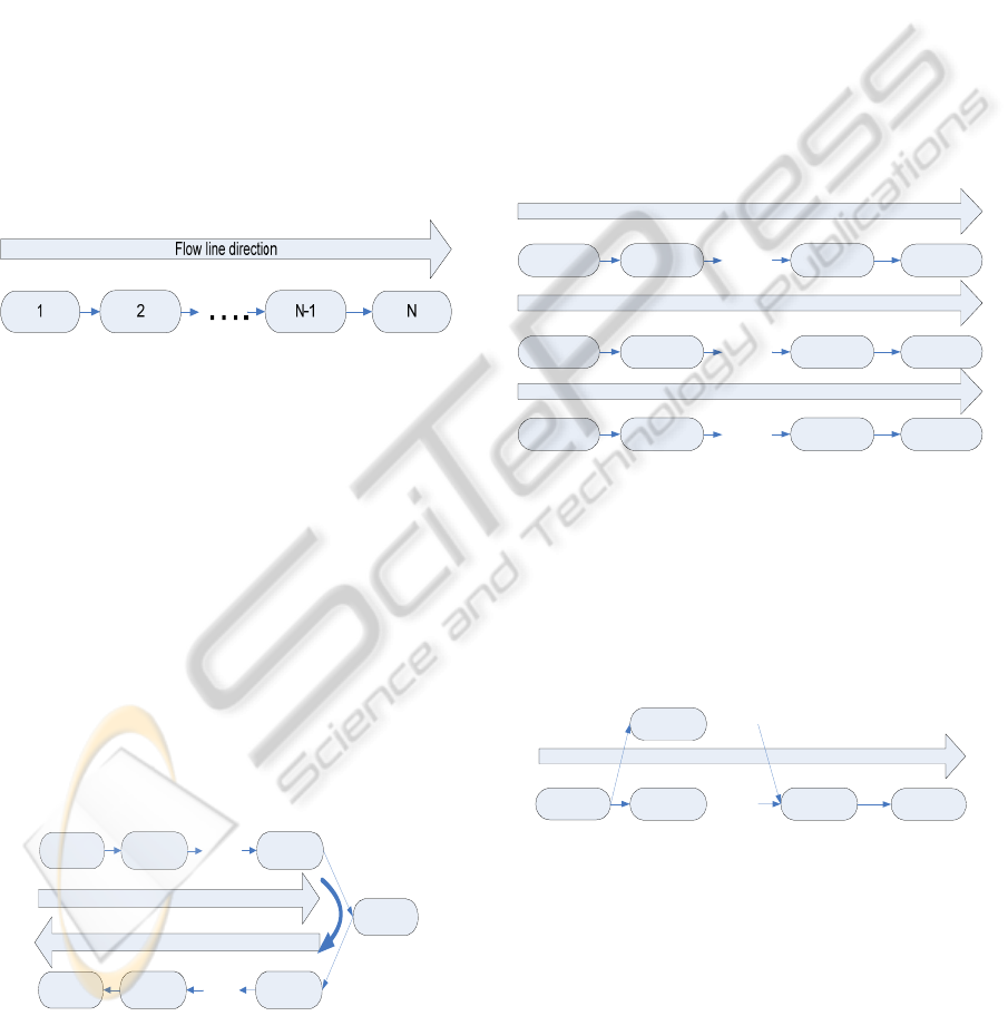
2.1 Serial (Single)
This is a very basic layout of a flow
is mostly used for small size products. These lines
have several disadvantages:
• monotone work,
• sensibility due to fai
• inflexibility due t
Figure 1: Serial line.
2.2 U-shape
ms of a serial line it
was redesigned to a form of U-shape (U-line). In
d Lines
In order to deal with the proble
such a line operators can work at more than one
station simultaneously. For example first operator
may both load and unload product units. As they are
included in more tasks during production process
they are gaining very important experience and
enlarge horizons. It is very helpful in case of just-in-
time production systems as it improves flexibility
which is crucial in dynamically changing demand
rates. What more, stations are closer together what
results in better communication between operators
and in case of emergency they are able to help each
other effectively.
1
2.3 Parallel Lines
In order to deal with problems described in case of a
serial line it might be a good idea to create several
lines doing the same or similar tasks.
Figure 2. U-line structure.
The advantages of such a solution (Sauer, 1997):
• increased flexibility for mixed-model
systems,
• flexibility due to changing demand rates,
• lowered risk of machine breakdown
stopping the whole production,
• cycle time can be more flexibly chosen
which leads to more feasible solutions.
The optimal number of lines is however a subject of
discussion for every single case separately.
2
M-1
M
…
.
N N-1 M+1
….
Flow line direction
Flow line direction
Figure 2: U-line structure.
1 2
N-1
N
….
Flow line direction
1 2 N-1 N
….
1 2 N-1 N
….
Flow line direction
Flow line direction
Figure 3: Parallel lines.
2.4 Parallel Stations
As an extension of serial lines bottlenecks are
replaced with parallel stations. Tasks performed on
parallel stations are the same and throughput is this
way increased (Askin and Zhou, 1997).
1
2
N-1
N
….
Flow line direction
….
2
Figure 4: Parallel stations.
2.5 Two-sided Lines
This kind of flow lines is mainly used in case of
heavy workpieces when it is more convenient to
operate on both sides of a workpiece rather than
rotating it. Instead of single working-place, there are
pairs of two directly facing stations such as 1 and 2.
As an example car line can be considered, and
mounting some parts like: side – doors (left, right
side), muffler (i.e. right side) or lights with no
ICINCO 2010 - 7th International Conference on Informatics in Control, Automation and Robotics
260

preference to the side. Such a solution makes the
line much more flexible as the workpiece can be
accessed either from left or right (Bartholdi, 1993).
In comparison to serial lines:
• it can shorten the line length,
• reduce unnecessary work reaching to the
other side of the workpiece.
1 3 N-3 N-1
….
Flow line direction
2 4 N-2 N
….
Figure 5: Two-sided line.
3 LOW MIX PRODUCT DEMAND
The volume of production is not a widely discussed
topic over the literature. There are numerous articles
about mixed-model assembly systems however they
do not investigate the problem of low product
demand. A formulation of a problem given in
(Bukchin et. al, 2002) should give an idea about it. J.
Bukchin indicates that it’s long gone, when
everybody was buying a black painted Ford T as
long as it was cheap. Back than, high productivity
was achieved by introducing a perfectly single
model with no additional features.
Nowadays, the life cycle of a product is relatively
short and the demand for varied product is high.
Consequently, a set of similar products needs to be
assembled in relatively low volume. The goal to
such an approach is flexible responding to shorter
product life cycles, low to medium production
volumes, changing demand patterns and a higher
variety of product models and options.
The conditions for such an installation are:
• assembly-to-order production,
• low product demand (low volume
production),
• number of tasks greater than number of
stations,
• lack of mechanical conveyance,
• Highly skilled workers.
It might be extended with conditions given by
(Heike et. al, 2001):
• flexible fixtures,
• flexible tooling,
• delivery of material.
Such conditions give a good base for an assembly
system robust to demand changes. Having a good
balancing algorithm is a goal in this case.
When the demand for a set of similar products is
insufficiently high in order to install a complete
assembly line a solution given in (Battini et. al,
2007) might be used. Most of the authors use
combined precedence diagrams in order to reduce
multiple models into a single model. As the plant
layout, they majority uses a straight line in some
cases allowing parallel workstations for omitting the
bottleneck effects. What more, some allow
duplicating stations in series. Authors investigation
U-shaped lines indicate their benefits over
traditional serial lines. Some of them are:
• improvement in labour productivity,
• job enlargement for human operators,
• great interaction between operators,
• reduction in number of required workstations,
• lead time contraction,
• increase of flexibility.
They suggest (Aase et. al, 2004) this kind of lines in
case of number of tasks less than 30 and 10 stations.
Fixed position layout should be taken into account
dealing with heavy workpieces as it is more
convenient to switch operators places rather than i.e.
rotating the part (Heike et. al, 2001). Generally,
when set-up times required between different
versions are significantly high a job shop layout
suits the best (McMullen, 2007).
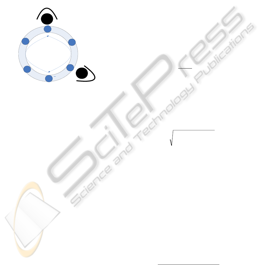
4 ASSEMBLY ROTATING ROUND
TABLE
The model and the procedure discussed in this
section bases on (Battini et. al, 2007). D. Battini
introduces a mixed-model assembly system
consisting of a rotating assembly table with a fixed
number of stations. It is a semi-automated system
therefore some stations are occupied by human
operators, some by machines and other are free.
Human operators are indicated by “O” while
automated ones as “A”. The resource assignment is
assumed to have no limitations, every operator or
machine can be placed at any station of the table.
The product assembled with such a system is
assumed to be homogenous with some additional
features that enable creation of joint precedence
diagram with known tasks’ durations. The rotating
table is a multi-turn one, as a matter of fact a batch
of one single product is completed in n number of
turns, with n ≥ 2. The table is an example of unpaced
ASSEMBLY SYSTEMS FOR LOW PRODUCT DEMAND - Estimation of Final Results
261

synchronous line controlled assembly system. It
means that all the tasks performed by operators need
to be completed before the shift of the table. It is
assumed that it has a pneumatic motion and all
operators need to press a button as an information
that they finished their task. If all the tasks are
finished the table switches their position with switch
time t
s
≥ 2s (move time between 2 stations). Every
switch of the table moves the workpiece to
following station – one station at each table switch.
1
2
3
4
5
6
OP1
OP2
Figure 6: Example of rotating assembly round table (two
human operators and six stations).
The assumption of rotating round table are:
1. The assembly rotating round table is multi-
turn type.
2. Precedence diagrams of all model types can
be accumulated into a single combined
precedence diagram.
3. The line production policy is “assembly-to-
order”.
4. Workpieces are fixed on the table and there is
only one workpiece at the station of the table
at a time.
5. Each station has only either one operator or
one actuator.
6. Idle operators cannot be used to help the
operators of other stations
7. The table switches only when all the opened
stations have finished their job.
8. The first task of the cycle is the load of all the
workpieces of the same batch on a table and
is always assigned to first operator.
9. The last task of the cycle is the download of
the assembled units and can be assigned to
any operator.
The objectives for this assembly system are:
1. Optimize the load balancing of each station
activated in the rotating table
2. Optimize the resource positioning in order to
minimize the entire make span of the
assembly batch, and consequently, the
average cycle time.
The goal of this paper is to compare serial assembly
system and rotating round table.
5 ESTIMATION OF FINAL
RESULTS OF BALANCING
PROBLEM
Some measures of solution quality have appeared in
line balancing problem. Below are presented three of
them (Scholl, 1998).
Line efficiency (LE) shows the percentage
utilization of the line. It is expressed as ratio of total
station time to the cycle time multiplied by the
number of workstations:
100%
Kc
ST
LE
K
1i
i
⋅
⋅
=
∑
=
()
(1)
where:
K - total number of workstations,
c - cycle time.
Smoothness index (SI) describes relative
smoothness for a given assembly line balance.
Perfect balance is indicated by smoothness index 0.
This index is calculated in the following manner:
∑
=
−=
K
1i
2
imax
STSTSI
(2)
where:
ST
max
= maximum station time (in most cases
cycle time),
ST
i
= station time of station i.
Time of the line (LT) describes the period of
time which is need for the product to be completed
on an assembly line
:
(
)
K
T1KcLT +
=
⋅
−
(3)
where:
c - cycle time,
K -total number of workstations.
The average cycle time for rotating round table is
calculated due to the formula:
K
X}t)]S(t{max[
Z
1lASk:k
k
sZK
Z
∑∑
=∈
⋅+
=C
(4)
where:
C – average cycle time,
t(S
k
) – station load,
ICINCO 2010 - 7th International Conference on Informatics in Control, Automation and Robotics
262

AS
Z
– set of stations activated in turn z,
Z – 1,..,Z are table runs,
K – total number of stations,
t
s
– switch time of the table,
X
k
– distance in switches between the major
load station and each activated in turn z.
6 NUMERICAL EXAMPLES
In this chapter an illustrative example of serial
assembly line and assembly rotating round table is
shown. An 8 tasks example of final product is
considered. In both cases for founding end solution
of balance a heuristic procedure (Update
Immediately First Fit – Number of Followers) was
implemented.
1
2
3
4 5 6
7 8
Figure 7: Precedence graph of numerical example.
Table 1: Operation time of numerical example.
Task i
Time t
i
Task i Time t
i
1 18 5 7
2 13 6 14
3 6 7 11
4 9 8 2
6.1 Serial Assembly Line
We consider serial assembly line with two workers it
means with workstation. It is a problem knows as
Simple Assembly Line Balancing Problem Type 2
when the number of stations is given and value of
cycle time is calculated.
1
N
i
i
t
c
K
=
⎡⎤
⎢⎥
⎢⎥
⎢⎥
=
⎢⎥
⎢⎥
⎢⎥
⎢⎥
⎣⎦
∑
(5)
where:
c – cycle time of serial assembly line,
t
i
– operation time of task i.
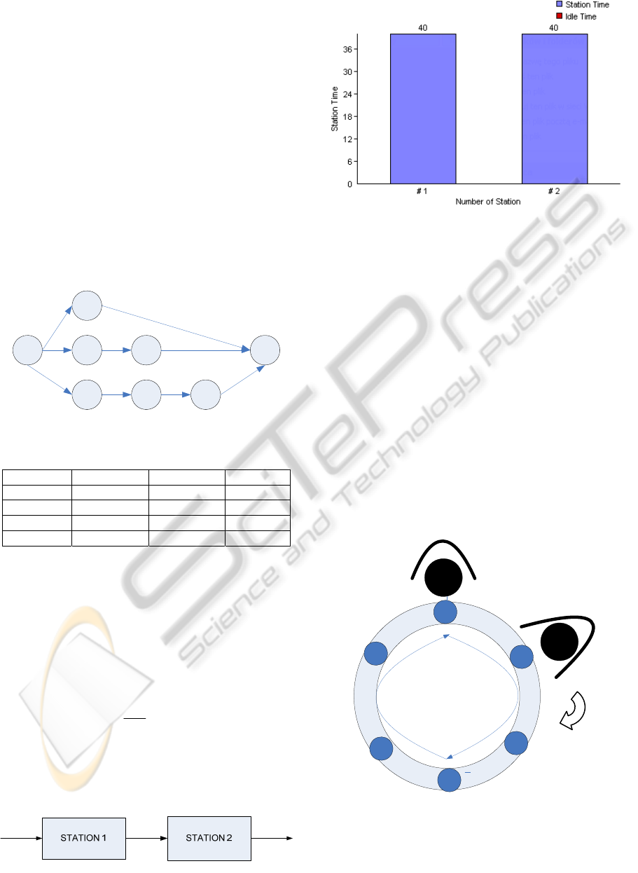
Figure 8: Serial two stations line.
Figure 9: Balance of serial line for calculated example.
The calculated cycle time is 40 (the total operation
time is 80) so we got final solution of balanced line:
Station 1 {1, 4, 3, 7) and Station 2 {5, 2, 6, 8). The
solution is optimal (mostly we obtain using heuristic
method only feasible solution) and calculated
measures are: SI = 0, LE = 100% and LT = 80).
6.2 Assembly Rotating Round Table
We consider now assembly rotating table with 2
human operators and six workstations. We obtain
final results for 6 cases it means we calculate
average cycle time for six different location of
human workers. Starting from position 1 and 2 we
relocate second operator to location 3, 4, 5 and 6.
Operator 1 is always assigned to station 1.
Relocation of Operator 2 causes that the distance
between both workers changes.
OP1
1
2
3
4
5
6
OP2
Figure 10: Location of human workers at assembly
rotating round table (1
st
case) and direction of movement.
Using heuristic described in (Battini et. al, 2007) we
obtained results which are presented in Table 2:
ASSEMBLY SYSTEMS FOR LOW PRODUCT DEMAND - Estimation of Final Results
263

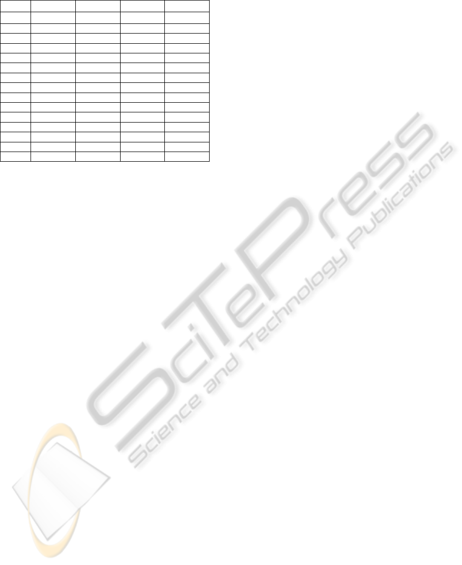
Table 2: Operation time of numerical example.
OP 1 OP2 Cycle Turns
1 Station 1 Station 2 53 2
2 Station 1 Station 3 61 3
3 Station 2 Station 3 53 2
4 Station 1 Station 4 56 3
5 Station 2 Station 4 61 3
6 Station 3 Station 4 53 2
7 Station 1 Station 5 58 3
8 Station 2 Station 5 56 3
9 Station 3 Station 5 61 3
10 Station 4 Station 5 53 2
11 Station 1 Station 6 70 2
12 Station 2 Station 6 58 3
13 Station 3 Station 6 56 3
14 Station 4 Station 6 61 3
15 Station 5 Station 6 53 2
The best average cycle time for assembly rotating
round table is 53 and it occurs always when
Operator 1 and Operator 2 are located next to other.
In this case we need to execute only two turns. The
final solution is: Operator 1 executes tasks 1 and 6
and Operator 2 executes tasks 2, 3, 4, 5, 7 and 8.
Additionally we can calculate the time when final
products is ready to unload from assembly system.
In our case the ready product leaves the system in
216 units of time. We should remember that
assembly rotating system is mostly effective in case
when product demand is equal to the total number of
stations.
7 CONCLUSIONS
In the paper two assembly systems were considered.
First assembly lines were presented. Next assembly
rotating round table was shown. The problems
seems interesting for low product demand. Known
procedures of solving balance of line structures
allow to get very easy optimal or near optimal
solution for two stations line. Investigated assembly
rotating round table allows to quick changes of
assembling different product. Heuristic procedure
improves the result of average cycle time from 70 to
53. This kind of assembly table takes benefits from
layout described in section 4 dealing with their
disadvantages such as monotony, boredom,
operators overload and communication. Different
measures of final result (smoothness index, line
efficiency, line time or average cycle time) simplify
the choice of the most appropriate solution. We
should underline that assembly rotating round table
system don’t need additional sequencing procedure.
Mixed product assembly deals with many
precedence relations but we choose only this one
with maximal number of tasks and connection.
Therefore we calculated the balance of whole model
with maximal task time operations. It allows to
choice appropriate cycle time of turn. In serial lines
we need to sequence the mix product model and
sometimes to stop the line (different model cycle
time) or to add additional parallel station.
This research was supported in part by grant of
Ministry of Science and Higher Education BK
209/Rau1/2009 t.5
REFERENCES
Aase, G. R., Olson, J. R., Schniederjans, M. J., 2004, U-
shaped assembly line layouts and their impact on labor
productivity: an experimental study, European
Journal of Operational Research, 156, 698–711
Askin, R. G., Zhou, M., 1997, A parallel station heuristic
for the mixed-model production line balancing
problem, International Journal of Production Research,
35(11), 3096-3106
Beker, C., Scholl, A., 2005, A survey on problems and
methods in generalized assembly line balancing,
European Journal of Operational Research, 168, 694–
715
Bartholdi J. J., 1993. Balancing two-sided assembly lines:
a case study, International Journal of Production
Research, 31(10), 2447-2461
Battini, D., Facio, M., Ferrari, E., Persona, A., Sgarbossa,
F., 2007, Design Configuration for a Mixed Model
Assembly System in Case of Low Product Demand,
The International Journal of Advanced Manufacturing
Technology, 34(1), 188-200.
Bukchin, J, Dar-El, M, Rubinovitz, J., 2002, Mixed model
assembly line design in a make-to-order environment,
Computers & Industrial Engineering, 41, 405-421
Heike, G., Ramulu, M., Sorenson, E., Shanahan, P.,
Moinzadeh., K, 2001, Mixed model assembly
alternatives for low-volume manufacturing: the case of
the aerospace industry, International Journal of
Production Economics, 72, 103-120
McMullen, P. R., 1997, A heuristic for solving mixed-
model line balancing problem with stochastic task
durations and parallel stations, International Journal
of Production Economics, 51(1), 77–190
Salveson, M. E., 1955. The assembly line balancing
problem, Journal of Industrial Engineering, 62-69
Scholl, A., 1998. Balancing and sequencing of assembly
line, Physica- Verlag
Sauer, G. A., 1998, Designing parallel assembly lines.
Computer Industrial Engineering, 35(3–4), 467–470
Sury, R. J., 1971. Aspects of assembly line balancing,
International Journal of Production Research, 9, 8-14
ICINCO 2010 - 7th International Conference on Informatics in Control, Automation and Robotics
264