A SUB-OPTIMAL KALMAN FILTERING FOR DISCRETE-TIME LTI
SYSTEMS WITH LOSS OF DATA
Naeem Khan, Sajjad Fekri and Dawei Gu
Department of Engineering, University of Leicester, Leicester LE1 7RH, U.K.
Keywords:
Linear prediction coefficients, Open loop estimation, Autocorrelation, Optimization.
Abstract:
In this paper a sub-optimal Kalman filter estimator is designed for the plants subject to loss of data or in-
sufficient observation. The methodology utilized is based on the closed-loop compensation algorithm which
is computed through the so-called Modified Linear Prediction Coefficient (MLPC) observation scheme. The
proposed approach is aimed at the artificial observation vector which in fact corrects the prediction cycle when
loss of data occurs. A non-trivial mass-spring-dashpot case study is also selected to demonstrate some of the
key issues that arise when using the proposed sub-optimal filtering algorithm under missing data.
1 INTRODUCTION
Loss of observation is a non-trivial case of study
in both control and communication systems. Such
loss may be due to the faulty sensors, limited band-
width of communication channels, confined memory
space, and mismatching of measurement instruments
to name but a few. Overcoming the side effects arose
from missing data in control and communication sys-
tems are remained as open research problems for re-
searchers during the last decade (Allison, 2001).
Perhaps, the best known tool for the linear esti-
mation problem is Kalman filtering (Khan and Gu,
2009b). However, Kalman filter depends heavily
on the plant dynamics, information of unmeasured
stochastic inputs, and measured data and hence it is
prone to fail if e.g., data is unavailable for measure-
ment update step. To overcome such shortcomings,
one approach for state estimation is to utilise the so-
called Open-Loop Estimation (OLE) when observa-
tions are subjected to random loss, see e.g. (Schenato,
2005; Liu and Goldsmith, 2004; Sinopoli and Schen-
ato, 2007; Schenato et al., 2007). They have stud-
ied LOOB cases, while running the Kalman filter in a
open loop fashion, i.e. whenever observation is lost,
the predicted quantities are processed for next itera-
tion, without any update.
More specifically, in OLE the prediction is based
on the system model and processed as state estima-
tion without being updated due to the unavailability
of the observed data. Nonetheless, in practice this
approach may diverge at the presence of longer loss
duration and it is likely that error covariance could
exceed the limits if the upper and lower bounds of er-
ror covariance are provided (Huang and Dey, 2007).
Another shortcoming of the OLE is the sharp spike
phenomena when the observation is resumed after the
loss. This is because the Kalman filter gain is set to
zero at the OLE during the loss time. But when ob-
servation is resumed, Kalman gain first surges to the
very high gains and then tries to approach the steady
state values in order to compensate loss impact. This
consequently results in a sudden peak to reach to the
normal trajectory of the estimated state which is not
a desirable behaviour for a reliable estimation algo-
rithm. Detail stability analysis of OLE can be found
in (Li Xie, 2007).
Under loss of observations for a longer period of
time, there is a requirement for an advanced estima-
tion technique which could provide superior estima-
tion performance under loss of data so as to maintain
the error covariance bounded. Our proposed approach
in this paper is based on an artificial optimal observa-
tion vector which is computed based on the minimum
error generated through the so-called Modified Linear
Prediction Coefficient (MLPC). Another advantage of
the proposed method is that it eliminates the spike of
the OLE technique.
(Micheli, 2001) has considered a delay in the data
arrival which may also be translated as lost or inac-
curate measured data. In (Schenato, 2005), a system
is assumed to be subjected to both LOOB and delay
of observation at the same time. All the above works
have suggested switching to an OLE estimator when
201
Khan N., Fekri S. and Gu D. (2010).
A SUB-OPTIMAL KALMAN FILTERING FOR DISCRETE-TIME LTI SYSTEMS WITH LOSS OF DATA.
In Proceedings of the 7th International Conference on Informatics in Control, Automation and Robotics, pages 201-207
DOI: 10.5220/0002953402010207
Copyright
c
 SciTePress

there is LOOB and a closed loop estimator when the
observation arrives at destination. This will aim in
fact at designing an estimator which is strongly time-
varying and stochastic in nature. In order to avoid
random sampling and stochastic behaviour of the de-
signed Kalman filter, (Khan and Gu, 2009b) has pro-
posed a few approaches to compensate the loss of ob-
servations in the state estimation through Linear Pre-
diction.
Throughout this paper we shall call the variables
in the case of loss of data as “compensated variables”,
e.g. P
{2}
k
is called the compensated filtered error co-
variance at time step k with loss of observation. The
rest of the paper is organized as follows. The theory of
the Linear Prediction Coefficient (LPC) is overviewed
in Section II. In Section III we discuss the proposed
sub-optimal Kalman filter with loss of data. The
mass-spring-dashpot case study is given in Section IV.
Simulation results are presented in Section V. Section
VI summarizes our conclusions.
2 THEORY OF LINEAR
PREDICTION COEFFICIENT
Linear prediction (LP) is an integral part of signal re-
construction e.g. speech recognition. The fundamen-
tal idea behind this technique is that the signal can be
approximated as a linear combination of past samples,
see e.g. (Rabiner and Juang, 1993). Whenever there
is the loss of observation, a signal window is selected
to approximate the lost-data. The weights assigned
to this data are computed by minimizing the mean
square error. These weights are termed as Linear Pre-
diction Coefficients. Out of the two leading LPC tech-
niques, (namely Internal and External LPC), we shall
develop and employ External LPC for LOOB, which
suits to our problem with constraints:
• The signal statistical properties are assumed to
vary slowly with time.
• Loss window should not be “sufficiently long”,
otherwise the prediction performance will be in-
ferior.
In this paper, the LP technique is termed as modi-
fied because in conventional LPC there is no defined
strategy to account the number of previous data, while
have defined several simple-to-implement algorithms
to decide that factor. One of it would be explain the
subsequent section.
Let us assume that the dynamics of the LTI system
is given in discrete time and that the data or observa-
tion is lost at time instant k. The LP is performed as:
¯z
k
=
n
∑
i=1
α
i
z
k−i
(1)
where ¯z
k
is called “compensated observation” and
′
α
′
’s represent weights of linear prediction coeffi-
cients for the previous observations and n denotes the
order of the LPC filter. Generally speaking, it depicts
the maximum number of previous observations con-
sidered for computation of compensated observation
vector. Also, n is required to be chosen appropriately
- higher value of n does not guaranty an accurate ap-
proximation of the signal but rather an optimal value
of n decides an efficient approximation and hence pre-
diction, see (Rabiner and Juang, 1993).
3 DESIGN OF SUB-OPTIMAL KF
WITH LOSS OF DATA
Let us assume that the process under consideration is
to be run by random noise signal whose mean and
covariance are independent of time, i.e. wide-sense
stationary process, given as
x
k
= Ax
k−1
+ Bu
k−1
+ L
d
ξ
k
(2)
z
k
= Cx
k
+ v
k
(3)
where A, B and C have appropriate dimensions, and
x, u, z, ξ and v are state, input, sensed output, plant
disturbanceand measurement noise, respectively. The
plant noise ξ and sensor noise v are assumed to be
zero mean white gaussian noises.
CKF computes the priori state estimation which is
solely based on (2). This priori estimation is thereby
updated with newly resumed observation at each time
instant. In the subsequent section, the performance of
CKF is tested and verified in a mass-spring-dashpot
system which help illustrate the proposed algorithm.
If the observation is not available due to any of the
reason mention earlier, the compensated observations
are calculated through (1).
The posteriori state estimation using this compen-
sated observation will be
¯x
k|k
= x
k|k−1
+
¯
K
k
(¯z
k
− ˆz
k
) (4)
The corresponding a posterior error for this estimate
is
e
k|k
= x
k
− ¯x
k|k
= x
k
− x
k|k−1
−
¯
K
k
(¯z
k
− ˆz
k
)
= e
k|k−1
−
¯
K
k
(¯z
k
− ˆz
k
) (5)
where x
k
is the actual state of the system. Conser-
vatively, the cost function of the Kalman filter is ob-
tained based on this a posterior error of the state esti-
mation.
ICINCO 2010 - 7th International Conference on Informatics in Control, Automation and Robotics
202

The optimal values of the modified linear pre-
diction coefficients (MLPC) are computed based the
residual vector as follows.
e
z
= ¯z
k
− ˆz
k
(6)
For the compensated estimation algorithm in MLPC,
our goal is to minimize the following cost function:
J
k
= E

e
T
z
e
z

= E

(¯z
k
− ˆz
k
)
T
(¯z
k
− ˆz
k
)

(7)
The MLPC are computed provided with the minimum
cost function i.e.
∂J
k
∂α
j
= 0 =
∂J
k
∂¯z
k
·
∂¯z
k
∂α
j
(8)
Performing simple and straight forward algebra the
above equation can be simplified as
E[ˆz
k
z
k−i
] −
n
∑
j=1
α
i
E{z
k+ j
z
k−i
} = 0
n
∑
j=1
α
i
E{z
k+ j
z
k−i
} = E[ˆz
k
z
k−i
] (9)
n
∑
j=1
α
i
γ
k
[i, j] = r
k
(i) (10)
or
R
k
· A
α.k
= r
k
A
α.k
= r
k
· R
−1
k
(11)
where
R
k
=





γ
k
(0,0) γ
k
(0,1) ··· γ
k
(0,n− 1)
γ
k
(1,0) γ
k
(1,1) ··· γ
k
(1,n− 1)
γ
k
(2,0) γ
k
(2,1) ··· γ
k
(2,n− 1)
.
.
.
.
.
.
.
.
.
.
.
.
γ
k
(n− 1,0) γ
k
(n− 1,1) ·· · γ
k
(n− 1,n− 1)





(12)
A
α.k
=




α
1
α
2
.
.
.
α
n




(13)
and
r
k
=




γ(1)
γ(2)
.
.
.
γ(n)




(14)
where E(z
k−i
z
k− j
) = γ
k
(i, j) and E(z
k
z
k− j
) = γ
k
( j) is
the autocorrelation function, which will be explain
shortly. Equation (11) requires inverting the ma-
trix of R
k
which may be increasingly difficult due
to computational demanding, especially at large or-
ders. To get rid of such burdensome calculations, sev-
eral attempts have been introduced in the literature.
Through Levinson Durbon or Leroux-Gueguen algo-
rithm the so-called ”Reflection Coefficients (RCs)”
are computed, which represent one-to-one linear pre-
diction coefficients. We shall explore and focus how
to calculate the optimal values of α
i
and n, when
the measurement contains a solid deterministic input
along with the unmeasured stochastic inputs. In prac-
tice, computing the autocorrelation coefficients need
extra attention. Generally, the autocorrelation coeffi-
cients are represented as
γ
m
=
C
m
C
0
(15)
where C
m
is the auto-covariance of y at lag m which
is
C
m
=
1
n− m
n−m
∑
j=1
(z
j
− ¯z)(z
m+ j
− ¯z) (16)
where ¯z =
1
n
n
∑
j=1
z
j
i.e. mean of the data for the se-
lected window. Without loss of generality, we shall
assume that that E(z
k
) = CE(x
k
) = D
k
.
A straightforward calculation would lead to the result
C
m
=
1
n− m
n−m
∑
j=1
(D
j
D
m+ j
) +
¯
D
2
−
¯
D
¯
D
m
−
¯
D
¯
D
M
(17)
and
C
0
=
1
n
n
∑
j=1
(D
2
j
) −
¯
D
2
+
1
n
n
∑
j=1
(v
j
)
2
(18)
where m ≤
n
2
and
D
j
= E(z
j
) = CE(x
j
)
¯
D
M
=
1
n− m
n
∑
j=m+1
D
j
¯
D
m
=
1
n− m
n−m
∑
j=1
D
j
¯
D =
1
n
n
∑
j=1
D
j
Clearly, one can observe that γ
0
=
C
0
C
0
= 1. And γ
1
=
C
1
C
0
< 1. Therefore, we can write
γ
0
≥ γ
1
≥ γ
2
≥ ··· γ
m
(19)
The inequality of (19) is an important equation which
helps in deciding the order of the LP filter as shown in
Algorithm-2. For better understanding of the descrip-
tive design, the measurement vector is written as
z
k
= η
k
(Cx
k
) + v
k
(20)
where η
k
is a random variable, such that
η
k
=

1, if there is no LOOB at time step k
0, otherwise
(21)
A SUB-OPTIMAL KALMAN FILTERING FOR DISCRETE-TIME LTI SYSTEMS WITH LOSS OF DATA
203

Therefore, the prediction step for the normal opera-
tion is as follows
x
k|k−1
= Ax
k−1|k−1
+ Bu
k−1
P
k|k−1
= AP
k−1|k−1
A
T
+ L
d
Q
k−1
L
T
d
(22)
The above predicted state and predicted state covari-
ance are achievable and remain unaffected with loss
of data. The conventional Kalman filter will update
the state and covariance on the arrival of observation
vector.This updated state and updated state covariance
are valid when there is no loss of data, i.e. system
is running in the normal operation. However, in the
presence of loss of measured data, the above standard
technique is failed. Toward this end, we have pro-
posed the closed-loop base MLPC algorithm, which
can also tackle the issues arising from data loss for
long period of time.
The Open loop estimator propagates the predicted
state and covariance without any update due to the
unavailability of the measurements as
x
{2}
k
= x
{1}
k
= Ax
{2}
k−1
+ Bu
k−1
P
{2}
k
= P
{1}
k
= AP
{2}
k−1
A
T
+ L
d
Q
k−1
L
T
d
(23)
While, in the proposed MLCP, the compensated ob-
servations are computed through 1 the modified linear
prediction scheme providing minimum error produc-
tion. The estimation produced by compensated obser-
vation is very comprehensive than those of open-loop
algorithms discussed earlier. The compensated obser-
vation are used to calculate compensated innovation
vector. Thereafter, the compensated Kalman gain is
computed as follows.
¯
K
k
=
¯
P
{1}
k
C
T
(C
¯
¯
P
{1}
k
C
T
+
¯
R
k
)
−1
(24)
Hence, the predicted state and covariance are updated
using this gain as
x
{2}
k
= x
{1}
k
+
¯
K
k
(¯z
k
−Cx
{1}
k
) (25)
P
{2}
k
= P
{1}
k
−
¯
P
{1}
k
C
T
(C
¯
¯
P
{1}
k
C
T
+
¯
R
k
)
−1
C
¯
P
{1}
k
The closed loop Kalman filtering algorithm is sum-
marized in Algorithm 1. There are various ways to
choose the value of the order of LP filter, n. Alter-
natively among these methods, we have found Algo-
rithm 2 very practical to be implemented in a number
of applications.
4 THE CASE STUDY EXAMPLE
The system under study in this paper is a slightly
modified version of a mass-spring-dashpot (MSD)
Algorithm 1: The proposed closed-loop estimation al-
gorithm using MLPC.
1: At time step: k− 1, Prediction is carried out as
x
{1}
k
= Ax
{2}
k−1
+ Bu
k−1
, and P
{1}
k
= AP
{2}
k−1
A
T
+
L
d
Q
k
L
T
d
2: Check: Status of η
k
if η
k
= 1
Run normal Kalman filter (obtain Filtered
Response i.e. x
k|k
and P
k|k
)
Else Obtain compensated filtered response (x
{2}
k
and P
{2}
k
) as mentioned below.
3: Select a suitable size for window (n) (No. of pre-
vious observations) and LP filter order (m) with
the constraint m < n/2
4: Construct autocorrelation matrix R
k
.
5: Construct modified residual matrix r
k
.
6: Compute MLPC through A
α.k
= R
−1
k
· r
k
7: Calculate compensated measurement vector as
¯z
k
=
n
∑
j=1
α
j
z
k− j
8: Obtain compensated residual vector
9: Calculate Compensated Kalman gain
¯
K
k
10: Measurement update step is carried out as:
x
{2}
k
= x
{1}
k
+
¯
K
k
(¯z
k
−Cx
{1}
k
): and
P
{2}
k
= P
{1}
k
− P
{1}
k
C
T
(CP
{1}
k
C
T
+
¯
R
k
)
−1
CP
{1}
k
:
11: Return to Step 1, i.e. repeat prediction cycle;
Algorithm 2: Selection of LP filter order.
1: Select γ
th
.
2: Compute γ
i
=
C
i
C
0
i = 1,2,···m
3: Check: Is γ
i
< γ
th
,
Yes Stop further computation of γ
i
m ← i and select order of LP filter as n =
2m+ 1.
Else
4: Compute i ←− i+ 1
5: Repeat Step 2
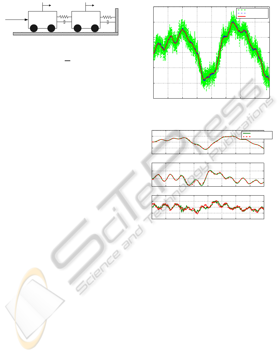
system given in (Fekri et al., 2007) as shown in Fig
1 which is a continues time system with dynmics as
follows.
˙x(t) = Ax(t) + Bu(t)+ Lξ(t)
y(t) = Cx(t) + θ(t) (26)
where the state vector is defined as
x
T
(t) = [
x
1
(t) x
2
(t) ˙x
1
(t) ˙x
2
(t)
] (27)
A =




0 0 1 0
0 0 0 1
k
1
m
1
k
1
m
1
−
b1
m1
b1
m1
k
1
m
2
−
k
1
+k
2
m
1
b
1
m
2
−
b
1
+b
2
m
2




(28)
ICINCO 2010 - 7th International Conference on Informatics in Control, Automation and Robotics
204

Control
u(t)
x
1
k
1
x
2
k
2
m
1
m
2
b
1
b
2
Figure 1: MSD two cart system.
B
T
= [
0 0
1
m
1
0
] (29)
C = [
0 1 0 0
] (30)
L = [
0 0 0 3
] (31)
The known parameters are m
1
= m
2
= 1, k
1
= 1, k
2
=
0.15 and b
1
= b
2
= 0.1 and the sampling time is T
s
=
1msec. Plant disturbance and sensor noise dynamics
are characterized as
E

ξ(t)

= 0, E

ξ(t)ξ(τ)

= Ξδ(t − τ), Ξ = 1 (32)
E

θ(t)

= 0, E

θ(t)θ(τ)

= 10
−6
δ(t − τ) (33)
After substituting the above known values the matri-
ces will be as follows:
A =



0 0 1 0
0 0 0 1
1 1 −0.1 0.1
0.1 −1.15 0.1 −0.2



(34)
and
B
T
= [
0 0 1 0
] (35)
In subsequent section, we will apply the proposed
MLPC algorithm to the above MSD system and show
some of the representative results. Many others were
also done but are not shown in this paper due to lack
of space.
5 SIMULATION RESULTS
Here we implement the above closed-loop MLPC al-
gorithm to the MSD system as discussed in Section
IV. For the purpose of our study, the continuous-time
dynamics of the MSD system is transformed to an
appropriate discrete-time model. Results depict the
performance of the Kalman filter when it is running
under the open loop i.e. during the period of un-
availability of observation, the prediction is not up-
dated and the predicted state and covariance are prop-
agated for the next time instant, see also (Khan and
Gu, 2009a). Figure 3 shows the performance of con-
ventional kalman filter via plotting the measured sig-
nal; x
2
, the position of Mass 2 with no loss of data.
0 500 1000 1500 2000 2500 3000 3500 4000
−30
−20
−10
0
10
20
30
Time (sec)
Movement of m
2
Conventional Kalman filtering for MSD without any Loss
Sensor Response
Filtered Response
Actual Response
Figure 2: Performance of CKF without data loss.
0 500 1000 1500 2000 2500 3000 3500 4000
−40
−20
0
20
40
Estimation of State
1
meter (m)
0 500 1000 1500 2000 2500 3000 3500 4000
−10
0
10
20
Estimation of State
3
m/sec
0 500 1000 1500 2000 2500 3000 3500 4000
−20
−10
0
10
20
Estimation of State
4
m/sec
Filtered Response
Actual Response
Figure 3: Other plant states.
Figure 4 shows three other states of the MSD plant
which again depicts the performance of conventional
Kalman filter when it is running normally, i.e. when
there is no data loss, for the rest three states (x
1
, x
3
=
v
1
and x
4
= v
2
), the position of Mass 1, the velocity
of Mass 1 and velocity of Mass 1, respectively. Fig-
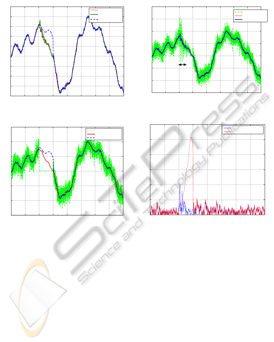
ure 5 shows the comparison analysis of the existing
open loop Kalman filtering and the proposed closed
loop MLPC algorithm based on compensated obser-
vation Kalman filtering. The sensor failure, namely
the loss of data, is introduced at 10–15 Secs. Fig-
ure 5 shows that the Open-Loop based estimation al-
gorithm diverges shortly and the estimation perfor-
mance is extremely inferior while the compensated
closed-loop observations generate satisfactory results
and better estimations. Figure 6 represents the Open-
Loop Kalman filtering along with measurements and
true sketch. During the loss, the observation value is
zero, and the predicted state which is taken as mea-
surement updated state is not following the true state
trajectory properly. Also, Figure 7 shows state esti-
A SUB-OPTIMAL KALMAN FILTERING FOR DISCRETE-TIME LTI SYSTEMS WITH LOSS OF DATA
205

0 500 1000 1500 2000 2500 3000 3500 4000
−20
−15
−10
−5
0
5
10
15
20
25
Time (sec)
meter (m)
Comparison of State Estimation by Compensated Estimation and Open−Loop
Actual Response
x
Est
by C/O
x
Est
by O−L
Figure 4: Comparison to two Estimation method.
0 500 1000 1500 2000 2500 3000 3500 4000
−30
−20
−10
0
10
20
30
Time (sec)
meter (m)
Estimation through Open Loop
Sensor Responnse
Actual Response
Filtered Response
Figure 5: State Estimation through Open-Loop.
mation through the proposed closed-loop. The mea-
surement vector is of higher magnitude but the update
state based on this higher value observation are much
better and comprehend. As a brief comparison, the
absolute error signals are shown in Figure 8. This er-
ror plots depict that priority of the proposed closed-
loop Kalman filtering MLPC over the previous open-
loop Kalman filter with loss of data. It is also true that
by providing the upper limit on the error bound, one
can notice that the data loss in the open-loop manner
will be very conservative than that of the close-loop
Kalman filtering.
6 CONCLUSIONS
We have presented a novel approach for state estima-
tion problem in discrete-time LTI systems subject to
loss of data. The approach exploits the artificial ob-
0 500 1000 1500 2000 2500 3000 3500 4000
−30
−20
−10
0
10
20
30
40
Time (sec)
meter (m)
Estimation by Compensated Observation
Sensor Response
Actual Response
Filtered Response
Figure 6: State Estimation through Closed-Loop.
0 500 1000 1500 2000 2500 3000 3500 4000
0
2
4
6
8
10
12
Time (sec)
meter (m)
Error Comparison of the two approaches
Error generated by CL
Error generated by OL
Figure 7: Error Comparison.
servation vector which in fact corrects the prediction
cycle when loss of data occurs, in order not to allow
the estimation error bounds to exceed the desired lim-
its. The resulting closed-loop Kalman filtering also
avoids the spike generated in OLE. The performance
of the proposed closed-loop Kalman filter approach,
when the prediction is updated with compensated ob-
servations, was illustrated via a mass-spring-dashpot
case study example.
REFERENCES
Allison, P. D. (2001). Missing Data. Sage Publications, 1st
edition.
Fekri, S., Athans, M., and Pascoal, A. (2007). Robust multi-
ple model adaptive control (RMMAC): A case study.
International Journal of Adaptive Control And Signal
Procession, 21:1–30.
ICINCO 2010 - 7th International Conference on Informatics in Control, Automation and Robotics
206

Huang, M. and Dey, S. (2007). Stability of kalman filtering
with markovian packet loss. Automatica, 43:598–607.
Khan, N. and Gu, D.-W. (2009a). ”Properties of a robust
kalman filter”. In The 2nd IFAC Conference on Intel-
ligent Control System and Signal Processing. ICONS,
Turkey.
Khan, N. and Gu, D.-W. (2009b). ”State estimation in the
case of loss of observations”. In ICROS-SICE Inter-
national Joint Conference. ICCAS-SICE, Japan.
Li Xie, L. X. (2007). ”Peak covariance stability of a random
riccati equation arising from kalman filtering with ob-
servation losses”. Journal System Science and Com-
plxity, 20:262–279.
Liu, X. and Goldsmith, A. (2004). ”Kalman filtering with
partial observation loss”. In IEEE Conference on De-
cision and Control, 43.
Micheli, M. (2001). ”Random sampling of a continuous
time stochastic dynamical system: analysis, state esti-
mation and applications”. Master’s thesis,, University
of Calfornia, Barkeley.
Rabiner, L. and Juang, B.-H. (1993). Fundamentals of
Speech Recognition. Prentice Hall International, Inc.
Schenato, L. (2005). ”Kalman filtering for network control
system with random delay and packet loss”. In Euro-
pean Community Research Information Society Tech-
nologies, volume MUIR, Italy.
Schenato, L., Sinopoli, B., Franceschetti, M., Poolla, K.,
and Sastry, S. S. (2007). Foundation of control and es-
timation over lossy network. Proceeding of The IEEE,
95(1):163–187.
Sinopoli, B. and Schenato, L. (2007). ”Kalman filtering
with intermittent observations”. IEEE transactions on
Automatic Control, 49(9).
A SUB-OPTIMAL KALMAN FILTERING FOR DISCRETE-TIME LTI SYSTEMS WITH LOSS OF DATA
207