MIXED COLOR/LEVEL LINES AND THEIR

STEREO-MATCHING WITH A MODIFIED

HAUSDORFF DISTANCE

Noppon Lertchuwongsa, Michèle Gouiffès and Bertrand Zavidovique

IEF, Institut d’ Electronique Fondamentale, CNRS 8622, Université Paris Sud 11, Paris, France

Keywords: Computer Vision, Stereovision, Color Lines, Hausdorff, Shape Matching.

Abstract: Level lines and sets are competitive features to support recognition. Color is assumed more informative than

intensity, so color-lines are preferred to exhibit the set basis. In the paper, they are defined after level lines,

and then extracted and characterize. Greater information is kept by color lines resulting into more efficient

grouping towards objects. A novel Hausdorff-inspired disparity finder is introduced fed in by color lines

with respect to epipolar constraints. The efficient disparity map resulting from pixel wise line-matching

between left and right images justifies our technical choices.

1 INTRODUCTION

Usual segmentation appears sensitive in practice to

the view point and shadows (contrast changes). In

this paper, morphologically stable sets are extracted

and a Hausdorff distance provides for global and

local pattern matching all in once. Level sets make a

basis - the topographic map - easy to compute.

According to psychologists (Koschan a Abidi

2008), in most contexts color prevails on shape and

texture: whence using color to make lines more

distinctive seems sensible.

Defining color sets and lines is not

straightforward because of the intrinsic tri-

dimensional nature of color. Usually, color data are

transformed from a 3D color space to a 1D Level

Space, by combining the three components, either to

specify a total order of colors or towards some

optimal function of those. Here, our of the

commonly used HSV space, the 1D level space is

provided by a mixture of H and V weighted by S.

After mixture line features have been extracted from

two images to compare, matching is carried out with

a coarse to fine strategy involving a modified

Hausdorff distance (Huttenlocher 1993), to pair

portions of lines.

As the disparity in stereoscopic images is

computed from the distance of corresponding points,

results of stereo shape matching and their

comparison with the ground truth will assert the

efficiency of our matching process, founding the

algorithm evaluation.

The paper is organized as follows. Section 2 is a

brief reminder on lines, color and matching for

notations and basic algorithms. Section 3 details our

procedure to enhance intensity lines into color lines.

Then, Section 4 deals with pattern and point

selections for matching towards disparity from line

pairing. Finally, the validity and efficiency of the

proposed procedure are evaluated through

comparing our depth map with the ground truth.

2 BIBLIOGRAPHY

Level sets and lines. Level sets (Caselles 1999), the

topographic map, prove invariant to contrast changes

and naturally robust to occlusions. Converting

images into sets and back is straightforward.

Projections follow equation (1) or (2)













)(,

xuxX

(1)

(2)

where u(x) is the gray level at pixel x in the image

and λ is the parameter – threshold – defining the

lower (resp. upper) set X

(resp. X

). reconstruction

follows equations (3)

(3)

A level line is the border of a level set, therefore

parameterized by the same λ. In practice it still

depends on the threshold’s step: as it is usually low





}{sup}{inf

Xλ,u=Xλ,u=xu 



122

Lertchuwongsa N., Gouiffès M. and Zavidovique B. (2010).

MIXED COLOR/LEVEL LINES AND THEIR STEREO-MATCHING WITH A MODIFIED HAUSDORFF DISTANCE.

In Proceedings of the 7th International Conference on Informatics in Control, Automation and Robotics, pages 122-127

DOI: 10.5220/0002948501220127

 SciTePress

valued in hope of an exhaustive topographic map,

images generate more lines than necessary to

matching. Color is likely to improve a priori the line

separability then lowering their number.

Color Edges and Lines. Color was first proved to

extend the notion of topographic map by (Coll &

Froment 2000) who designs a total order in the HSV

space. Gouiffès (2008) proposed to extract color sets

from color bodies in the RGB 3-D histogram.

Moreover the Hue in HSV proves ultimately

discriminative and invariant to shadow, however it is

ill-defined at low saturation. Compared to gray level,

color provides more edge or line information.

Feature matching. Set-correspondence finding

between two images can be classified into three

principal algorithmic lines: Point matching, based on

correlation windows on raw intensity data, but suffer

on homogeneous areas. Geometrical Feature

matching are the corners or curvature points or line

segments with attributes. Region and shape

matching strategies. The hypothesis is made here

that corresponding patterns maintain the shape

between images (Loncaric 1998).

The method we detail in the present paper

exploits the shape stability granted by the invariance

to contrast through color sets.

3 COLOR SETS AND LINES

3.1 Color Sets

Color image data can be represented in the RGB

cube. The pixel intensity – i.e. level – amounts to

projecting the given RGB point onto the principal

diagonal of the cube (the gray level scale). The

question then arises to find a transformation more

adaptive to the image content. Gouiffes &

Zavidovique (2008) proposed to use the dichromatic

model to find body colors: vectors pointing to

principal body colors are used separately instead of

the sole cube diagonal. Related data – i.e. close

enough in the RGB space – is projected onto that

vector exhibiting associated level sets.

Our leading idea to build the transformation of

the HSV color space into a 1-D level space takes

after the vanishing of Hue, independently at both

low light intensity and low saturation.

3.2 H,V Mixtures vs. S

Considering the above-mentioned drawbacks of the

HSV space, the following formulation of S is

preferred:

(,,) (,,)S=MaxRGB MinRGB



(4)

Second, we propose to use hue when it is

relevant(high saturation) and intensity otherwise

(low saturation). To ensure color sets homogeneous

enough respective to what is expected from regions

in image segmentation, we design a smooth

transition with a sigmoid function Sig(s,k):

() (,) () (1 (,))()

Op SigskHp SigskIp





(5)

Sig(s,k) is thus parameterized by its slope s and

inflection point k to be adapted from former  and 

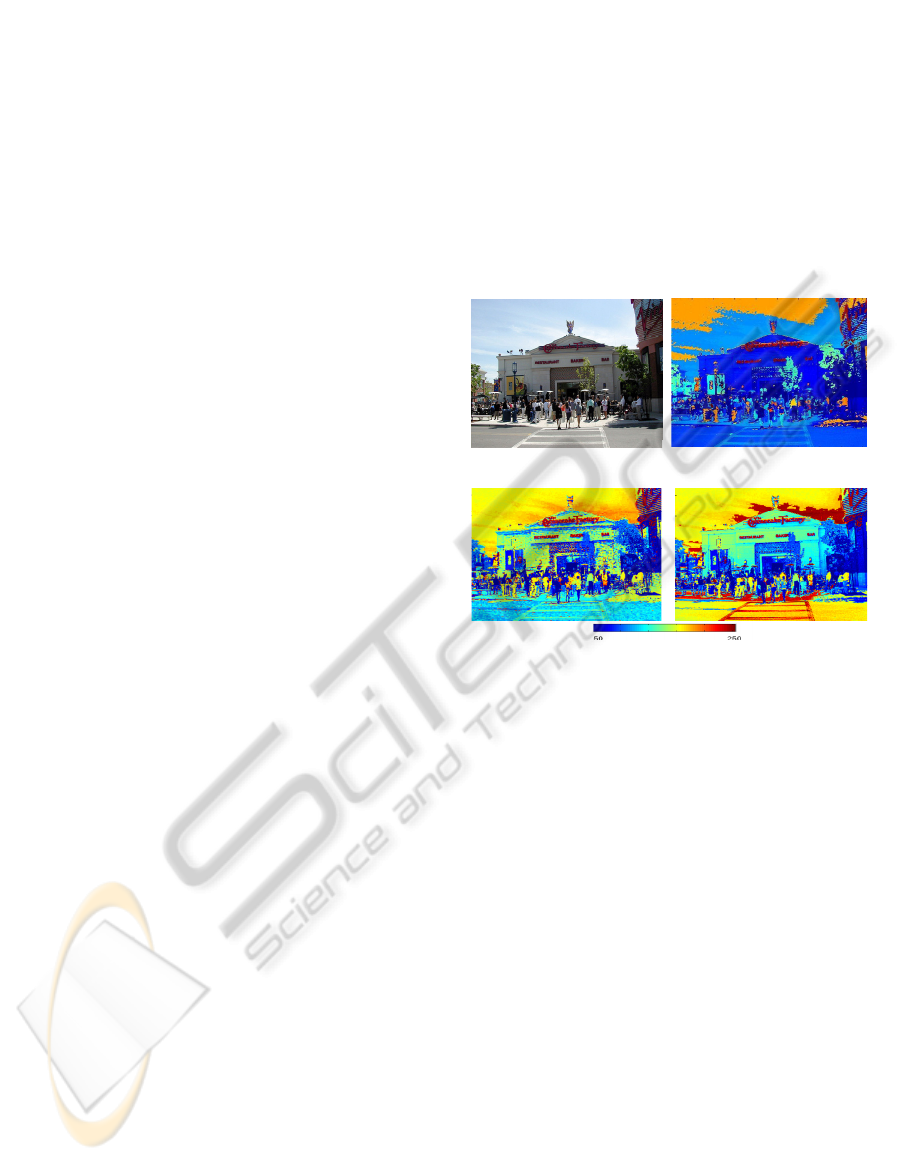
Figure 1: (a) Original image, (b) pseudo-color image in the

data space from the step function O

and threshold on

intensity, (c) pseudo-color image in the data space from

the sigmoid mixture O

and a threshold on intensity, (d)

pseudo-color image from the same data space and a

threshold on magnitude of the saturation, both (b) (c) and

(d) use same scale of pseudo color.

Fig 1 compares the use of a sigmoid (Fig. 1(c)) is

compared with the use of a Heaviside step function

(see Fig 1 (b)). On top of regular noise, the artifacts

of the step function are likely due to the frequency

of switches between the intensity and hue scales

when saturation lies in around the threshold. The

overall consequence is a loss of some details when

trying to lower the effect. The drawback of the

sigmoid function, compared to the step function, is

conversely its smoothness. When saturation is low,

although hue does not keep much of an effect, a

change of the RGB vector even to a close one might

result into significant modification of the final result

due to the small signal situation. Pepper noise

can occur on the image during the transition of the

Sig function around point k. Fig.1(c) finally

illustrates that issue: for example, on the road area,

the wall of the restaurant, or among the crowd, the

(a) (b)

MIXED COLOR/LEVEL LINES AND THEIR STEREO-MATCHING WITH A MODIFIED HAUSDORFF DISTANCE

123

sigmoid combination outputs some sparse noise.

Sharpening the sigmoid to make it closer to a

step function will reduce details. Since, again, the

sigmoid is more biased by the hue and is exactly

used to take advantage from it, the inflection point k

is set to a low value. Figure 1(d) shows better results

in that respect thanks to replacing the usual formula

of the saturation – a ratio – by the difference version

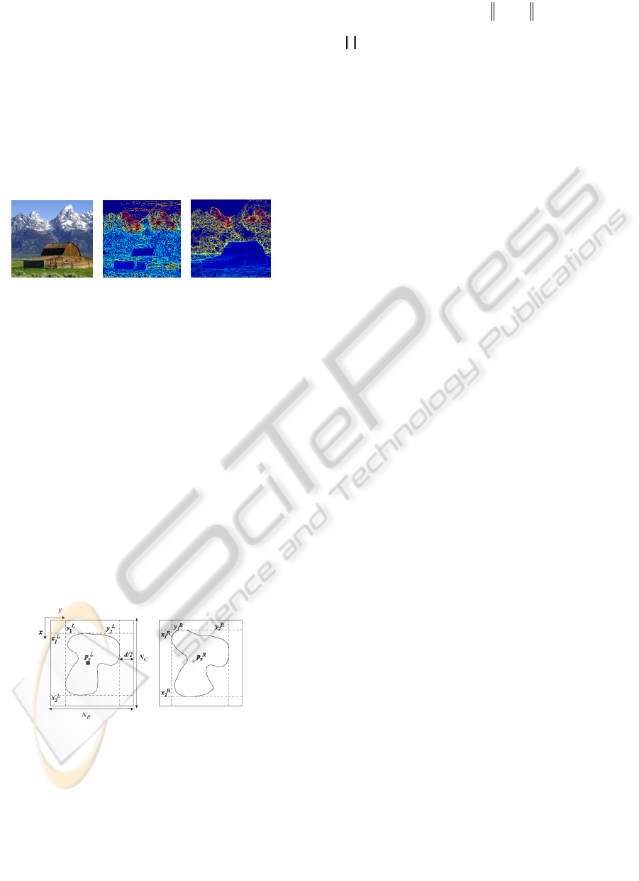
given in equation (4). Finally, Fig. 2 compares our

lines with the classical gray level lines.

Our line extraction method derives from the one

proposed by Bouchafa (2006) to direct close curve

extraction.

(a) (b) (c)

Figure 2: (a) Original color image, (b) gray level lines, (c)

color lines. Note that (b) and (c) result from a same

artificial look-up table to make lines more distinct.

4 COLOR LINE MATCHING

To speed the match up, our method begins to sort

patterns by global features for a coarse stage. Then,

at the fine stage, point matching is performed.

Coarse Scale Matching. Techniques of comparing

border of sets between 2 shapes, such as, length,

level of set, standard deviation and position shape,

which is exploited from stereo vision knowledge.

Fine Matching. Published techniques relying on a

reference point, e.g. Chang (1991), strongly depend

on this point stability.

(a) (b)

Figure 3: Example of corresponding sets A and B and their

centroids and notations.

The Hausdorff distance founds an interesting

technique to get the process free from the center. Let

A = {a

,...,a

} and B = {b

,...,b

} be two finite sets.

Their Hausdorff distance is defined as

 





A,B = Max h A,B ,h B, A

(6)

where





aA bB

hA,B=MaxMina b





(7)

and is a norm in the affine space of the image.

In previous works, e.g. (Huttenlocher 1993)

Hausdorff was used to locate shapes in a scene by

using a template.

Here, a topographic map contains abundant lines

which are close together, hampering the accuracy of

the distance map in our application. Therefore a

progressive scheme is rather tried: every tentative

couple of left and right lines is extracted and

superimposed within a common window W with

center p

of coordinates (x

, y

) and of size N

. However, using the center of W, p

= (N

/2,

/2) as the reference point for mapping, two

problems occur. First, direct mapping of the centroid

of W may make some part to exceed the window.

Second, right and left patterns to be matched can be

dissimilar since they were filtered roughly, therefore

large enough space d is needed to compensate.

Thus, a slightly more elaborated shifting strategy

into W has to be designed (see Fig. 3). x

, x

, y

are the coordinates of the bounding rectangle of

the left pattern, and p

= (x

, y

)

is the centroid

(small square) of the line to be mapped in the

comparison. It is likely different from the center of

the window, illustrating the first problem.

Finally, both each point p

= (x

, y

) of L

and

each point p

=(x

, y

) of L

are translated into W, of

reference point p

= (xc

, yc

) and of size N

x N

respectively with vectors v

and v

cRWRWRR

cLWLWLL

yyxxwith

),('''



vvpp

(8)

(9)

where The new centroid p

is then defined as:











































)/()(

121

LLLL

yyyy

xxxx

(10)

(11)

and comparison window is the rectangle N

x N

dyyN

dxxN



(12)

(13)

where d is the extension of the window from the size

of the line

Note that, according to the stereovision

application targeted in our paper, we assume that the

epipolar constraint holds, Therefore, the translation

on row x is similar in v'

and v'

. This assumption

reduces significantly the complexity of the

Hausdorff matching so made one-dimensional. After

shifting the selected left line L

to W (equation (8))

ICINCO 2010 - 7th International Conference on Informatics in Control, Automation and Robotics

124

the distance map is computed with a city block

distance. Then, candidate samples of right lines are

mapped to W – equations (8,9) – and the Hausdorff

distance is computed for all right line candidates in

as resulting from the coarse scale matching. The

final homologous line is the line which provides the

minimum Hausdorff distance - equation (6) .

Indeed, when finding the point-to-point or line-

to-point distances, we use their minimum. Pattern-

to-pattern distances, i.e. set of points to set of points,

result from the furthest of those closest points. When

a pattern is selected by the Hausdorff’s condition, all

points in the set will find their corresponding part.

is the translation vector bound to the

minimum Hausdorff distance (see Fig. 4), and d

the local Hausdorff vector between corresponding

columns of points p'

and p'

(respectively y'

and

). The disparity D of corresponding points p

and

is obtained from the stereo pair, following:

dTp 

RLL

yyyyD )(

(14)

Note that the disparity value is computed at all

sample points of a line.

(a) (b)

Figure 4: (a) Right line L

(dotted line), superimposed on

(continuous line) when L

was firstly projected into W

which already had L

as distance map, centroid of L

marked as

. (b) The Hausdorff method makes L

translate to new centroid

= p

. Finally, the vector

goes from p'

to p'

Decomposing Lines. A single global distance to all

points corresponds to a simple linear transformation

between homologous points. Indeed, one region or

line can relate to several depths. Also, one line likely

refers to several objects at different depths. Rather

than a complicate set of equations, the line can be

decomposed into portions where the rigid motion

applies well enough.

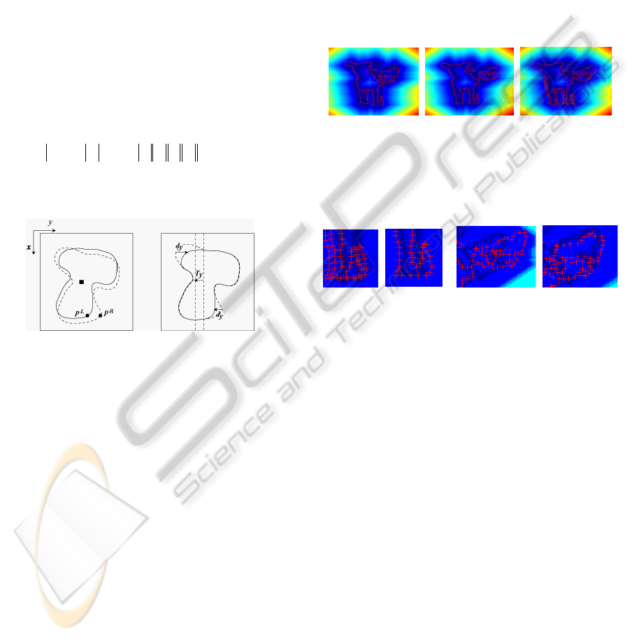
In figure 5, the line points extracted from the

right image of a stereoscopic pair (red crosses)

superimpose with the left line from the distance

map. Blue means close and the redder the further.

Let us call "centroid match" the process where

the two centroids are superposed first and then the

result for every pair of corresponding points is

computed.

In fig.5 (a) the centroid match leads to large

distances between corresponding points, up to

missing corresponding points on the right border of

the right leg (reader’s right) that are paired with the

left border of the right leg. In Fig. 5(b) Hausdorff

makes both lines have correct co-points, generally

better than before. The distance of corresponding

points is reduced; however there are still some

misfits in the tail (right area of the deer). Finally,

Fig. 5(c) illustrates our technique. Obviously, the

number of mismatched points was efficiently

reduced. Fig. 6 shows some enlarged details of the

points matching.

(a) (b) (c)

Figure 5: Illustration of the matching procedure. Right

lines' (Red Cross symbol) superimposed on left lines'

distance map (dark). (a) lines based on the same centroid

at the center window, (b) lines after optimal Hausdorff

translation, (c) result of the proposed method.

(a) (b)

Figure 6: (a) Enlarged version of the leg part in figure 17:

left, centroid matching; right, modified Hausdorff. (b)

close up on the tail part of figure 17: left, general

Hausdorff, to compare with right, modified Hausdorff.

5 EXPERIMENT AND RESULTS

Color lines are evaluated first in comparing with

gray level lines. They are then used to evaluate the

efficiency of the modified Hausdorff distance. This

distance is compared to classical line matching

methods through the stereo matching quality for

both color and gray lines. The database, 2003-2006,

Scharstein (2003, 2007) and Hirschmüller (2007) is our

test bench.

5.1 Contribution of the Color Lines

The relevance of our color mixture lines wrt. gray

level lines, is indicated by two criteria: 1) the

number of lines, compactness of the topographic

map. 2) The average PSNR values and number of

lines computed on the image data base are collected

in the table 1. Three different data are considered:

MIXED COLOR/LEVEL LINES AND THEIR STEREO-MATCHING WITH A MODIFIED HAUSDORFF DISTANCE

125

gray, abrupt mixture, and sigmoid.



is the

quantization step, both PSNR and “line number” are

decreasing functions of



. k sets the mix (section 3).

From the analysis of the table 1, we can note that

the PSNR for the sigmoid mixture is lower than with

Gray lines except when the saturation is greater than

or equal to 0,4. The number of lines is appreciably

lower in same conditions. That means images

reconstructed from a topographic map after smooth-

mixture are closer to the input image, while the

topographic map is more compact. Fig. 7 shows

examples of level and color sets.

Table1: Comparison results between images after color

mixture data and gray level ones: average PSNR of each

kind of data and the average number of lines.



PSNR

Gray 1 - 42.33 36474.30

2 - 37.97 29234.31

5 - 31.19 18666.96

0.1 36.46 29378.13

0.2 38.15 30617.52

0.4 42.53 33416.48

0.1 32.63 20784.17

0.2 34.41 22332.59

0.4 38.68 25575.09

0.1 27.97 11498.09

0.2 29.77 12779.41

0.4 33.51 15507.00

Nb. lines .

Sigmoid method

Figure 7: Examples of level and color sets: (a) Original

color image, (b) Pseudo color image of gray level sets, (c)

Pseudo color image of sigmoid color set: for all pseudo

color images the step parameter is set equal to 5, the

amplitude is coded on 8 bits and k = 0,2 for the mixture.

Line images are shown in Fig. 8. As expected, many

lines appear on colorimetrically homogeneous

objects. Shadows produce lots of irrelevant lines,

unstable for matching since they do not correspond

to real objects. With the sigmoid mixture, the

topographic maps are more compact and lines

correspond to salient physical items at sight.

This preliminary experimental evaluation

suggests that our HSV mixture produces lines more

appropriate for matching, i.e. more distinctive,

quicker to compute, and more related to object-

boundaries.

5.2 Matching Results

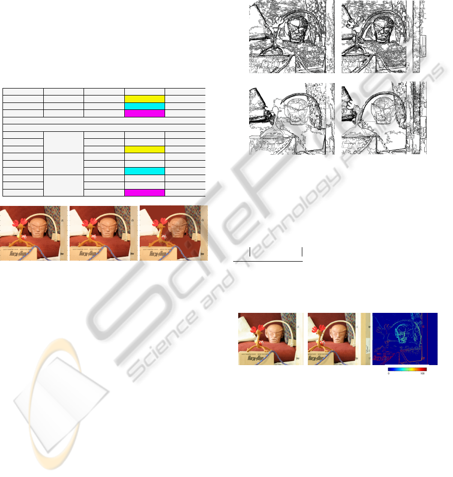
Figure 9 shows an example of results of our

disparity computation method and figure 13 displays

the error from the ground truth in every pixel. Most

matching errors occur for large color lines related to

several objects at different depths.

In Table 2 , N

refers to the average number of

line points computed in the whole data base. N

the number of correct points, those for which the

disparity error is less than 5. E

stands for the mean

disparity error computed on the N

points and E

same on the N

points.

(a) (b)

Figure 8: Examples of lines from the stereo pair of Fig.7.

Step

 is set to 2, and the inflection point k is 0.2. (a), (b)

are the gray level lines in left and right images

respectively, (c) (d): Lines from sigmoid mixture.

The parameter %D

E>5

(resp.%D

E>1

) is the

percentage of points with a disparity error









x, y D x, y





greater than 5 pixels (resp. 1

pixel), D

(x,y) being the disparity after our method

at pixel (x,y) and D

(x,y) the truth after the data

base; n is the number of pixels.

(a) (b) (c)

Figure 9: Example of matching: (a), (b) left and right

stereoscopic images, (c) the disparity-line image and its

color map value.

These criteria are computed for the Hausdorff

distance and the centroid method. The Hausdorff

method is used with gray and Sigmoid Mixture data

(the parameter that we use is T

= 0.2). Out of table

2, gray level data yields a larger number of points

than the mixture in same technical conditions.

Most added points are not salient and those from

shadow lines are unstable. Consequently, 19,3% of

the gray lines have not been correctly matched,

ICINCO 2010 - 7th International Conference on Informatics in Control, Automation and Robotics

126

compared to only 13 % for the mixture lines. Too

large a number of lines is also problematic in terms

of computation times and resources. Eventually,

disparity errors are always lower from mixture lines.

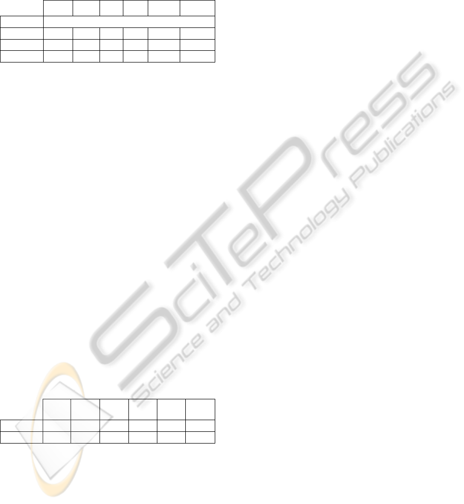
Table 2: Comparison of the results provided by the

Hausdorff matching and classical centroid line matching.

E>5

E>1

Hausdor

Gray

6092 497

4,9

0,7

18 54

Mixture

3585 313 4,0 0,6

13,51 50,63

Centroid

3892 289 6,9 1,0

28,07 67,73

For comparison purposes, Table 2 collects also

results from the Centroid technique on mixture data.

is normalized to find a number of lines

comparable to Hausdorff’s by controlling the T

threshold of acceptable data as defined in section 4.

Even if T

is adjusted in the Hausdorff case, it could

only worsen results since the matching condition

states that a tighter threshold means more similar

patterns. T

depends on the line length not on the

type of input data. Then on the same image sub-part,

26,6 % of the lines have not been correctly matched.

Moreover, the errors E

and E

are significantly

higher than Hausdorff ‘s (E

: 69% and E

: 59%).

The same N

value is kept for gray vs. mixture

lines not to bias results (same technique and

parameters).

Contribution of the Modified Hausdorff Distance.

Table 3 compares the classical and modified

Hausdorff distances for the color mixture. In the

latter case, lines are divided if their length is higher

than an experimentally set threshold T

, the value of

which depends on the image size through natural

stretching and shrinking in stereo (T

=500 in our

experiments). Same measures as before are collected

Table 3: Comparison of classical Hausdorff techniques

and modified techniques.

E>5

E>1

Classical 23185 18621 3,5744 1,0840 21,01 65,53

Modified 24585 21357 3,1402 0,8753 14,22 60

Because these techniques are based on a different

Hausdorff matching, the threshold of acceptable data

Ta is separately chosen to reach the same level of

details in the disparity image.

According to table 3, the classical Hausdorff

method yields a smaller number of points which

means less detail compared to the modified

Hausdorff. It produces even a smaller number of

points, N

, for which the disparity error is less than

5. Nevertheless, the average error E

(Column 4) is

3,57 pixels for the global Hausdorff and only 3,14

pixels for the modified version. Likewise, the rate

E>5

in column 5 is 21,01% vs.14,22%, meaning

that 79% of the lines are correctly matched by the

classical approach, while 85,8% are correctly

matched with the modified version. And finally,

Table 3 also shows that the disparity errors are

always lower with the modified Hausdorff distance.

6 CONCLUSIONS

Our work studies color line matching and evaluates

its relevance in a stereo matching application. A

novel color topographic map is proposed with less

irrelevant lines, more related to objects and more

distinctive. Direct close curve extraction based on

the color map reduces the memory and CPU greed.

Color sets finally prove more stable in practice than

usual results of region segmentation. The proposed

modified Hausdorff shows its efficiency in finding

more accurate correspondences for image

registration.

REFERENCES

Koschan & Abidi (2008). Digital color image processing.

Hoboken, N.J.: Wiley-Interscience.

Huttenlocher, Klanderman & Rucklidge (1993).

Comparing images using the Hausdorff distance.

IEEE Trans. on PAMI, Vol. 15. N° 9. pp. 850–863.

Caselles, Coll & Morel (1999).Topographics maps and

local contrast invariance in natural images. IJCV, pp.

5-27.

Coll & Froment (2000), Topographic Maps of Color

Images. In ICPR Vol. 3. p 3613. 2000.

Gouiffès & Zavidovique (2008), A Color Topographic

Map Based on the Dichromatic Reflectance Model.

Eurasip JIVC, n.17.

Loncaric (1998). A survey of shape analysis techniques.

Pattern Recognition Vol. 31, pp 983-1001.

Bouchafa & Zavidovique (2006) Efficient cumulative

matching for image registration. IVC, Elsevier Vol.

24, pp.70-79.

Chang, Hwang & Buehrer (1991) A shape recognition

scheme based on relative distances of feature points

from the centroid, Pattern Recognition, Vol. 24, N°11,

pp. 1053-1063.

Scharstein & Szeliski (2003). High-accuracy stereo depth

maps using structured light. In IEEE CVPR Vol. 1,

pp. 195-202.

Scharstein & Pal (2007). Learning conditional random

fields for stereo. In IEEE CVPR.

Hirschmüller & Scharstein (2007). Evaluation of cost

functions for stereo matching. In IEEE CVPR.

MIXED COLOR/LEVEL LINES AND THEIR STEREO-MATCHING WITH A MODIFIED HAUSDORFF DISTANCE

127