A CONSTRAINED FINITE TIME OPTIMAL CONTROLLER FOR

THE DIVING AND STEERING PROBLEM OF AN AUTONOMOUS

UNDERWATER VEHICLE

George Nikolakopoulos, Nikolaos J. Roussos

Hellenic Navy Research Center (GETEN), Ministry of Defence, Papagos, Athens, Attika, Greece

Kostas Alexis

Department of Electrical and Computer Engineering, University of Patras, Rio Achaias, Greece

Keywords:

AUV, Constrained ﬁnite time, Optimal control.

Abstract:

In this paper a Constrained Finite Time Optimal Controller (CFTOC) is designed and applied to the diving and

steering problem of an Autonomous Underwater Vehicle. The non–linear model of the AUV is presented and

the decoupled linear models for the steering and diving motions of the vehicle are derived, based on certain

modeling assumptions and simpliﬁcations, while the cruising speed of the vehicle is considered to be small

and constant. The proposed control scheme has the merit to take under consideration: a) the mechanical and

physical constrains of the AUV, b) uncertainties produced from modeling errors and environmental noise, c)

constrains in the motors, and produce an optimal controller for the vehicle that will guarantee the stability of

the closed loop system. Theproposed CFTO–controller is applied to simulation studies and relevant simulation

results are presented that prove the efﬁcacy of the proposed scheme.

1 INTRODUCTION

In the last years there was a strong interest towards

the development of Autonomous Underwater Vehi-

cles (AUV) and Remotely Operated Vehicles (ROV).

These classes of underwater vehicles are intended to

provide simple, long–range, low–cost measurements

of environmental data or surveillance studies. Al-

though ROVs have been utilized in the past in many

applications, in the recent years there has been a

growing demand for the utilization of AUVs as these

vehicles are superior to the ROVs, are completely au-

tonomous and are not suffering from the demand of

high operating costs, dedicated cables for carrying the

data links between the vessel and the ROV and expe-

rienced crew to guide the vehicle (Yuh, 2000; E. An,

2001; Foresti, 2001).

The superiority of AUVs and their complete au-

tonomy are generating more demands for modeling

approaches and applied control algorithms as more

accurate and fast control actions should be applied to

the vehicle to improve the overall performance. In

the utilized model of an AUV, when other factors are

taken under consideration, including: a) parametric

uncertainties such as added mass, hydrodynamic co-

efﬁcients, lift and drag forces, b) highly and coupled

non linearities, and c) environmentaldisturbances like

ocean currents and wave effects, the problem of ap-

plying a most suitable control law is widely increased.

In the area of mathematical modeling for AUVs,

there have been extended analytical approaches with

the main variation being the level of association be-

tween the hydrodynamic phenomena and the under-

water rigid body dynamics. In the general case the

mathematical models contain hydrodynamic forces

and moments expressed in terms of a set of hydro-

dynamic coefﬁcients, therefore it is of paramount im-

portance to a priori know the true values of these

coefﬁcients to control the AUV accurately. In most

of the cases experimental measurements are needed

to tune the hydrodynamic parameters of the models

while the relative literature is providing sufﬁcient ref-

erences and methodologies for calculating these pa-

rameters in various types of underwater vehicles.

In the area of controlling AUVs, until now various

classical approaches have been utilized. More specif-

ically many control strategies have been appeared in

260

Nikolakopoulos G., J. Roussos N. and Alexis K. (2010).

A CONSTRAINED FINITE TIME OPTIMAL CONTROLLER FOR THE DIVING AND STEERING PROBLEM OF AN AUTONOMOUS UNDERWATER

VEHICLE.

In Proceedings of the 7th International Conference on Informatics in Control, Automation and Robotics, pages 260-267

DOI: 10.5220/0002948202600267

 SciTePress

the literature for the diving and steering control of an

AUV such as: Optimal control (Field, 2000), Neu-

ral Networks (Kawano and Ura, 2002), Fuzzy con-

trol (Debitetto, 1995), Adaptive Sliding Mode con-

trol (Cristi et al., 1990), Proportional and Derivative

(PD) control (Bjorn, 1994; Pestero, 2001), Sliding

Modes Control (SMC) (Healey and Lienard, 1993;

Rodrigues et al., 1996) and Linear Quadratic Gaus-

sian (LQG) controller (Fossen, 1994b). In all these

approaches, in the ﬁrst stage of the controller design,

decoupling can be applied to the movements of the

AUV and each movement can be modeled and con-

trolled by a different set of differential equations and

different controllers.

In the current research effort the aim is to utilize

a more accurate and realistic modeling approach for a

torpedo like AUV, the REMUS AUV, and based on the

derived decoupled model of the vehicle’s motions to

design a novel constrained ﬁnite time optimal control

scheme for the diving and steering motions. The pro-

posed control scheme has the advantage of taking un-

der consideration in the design phase: a) the physical

and mechanical constrains, b) the disturbances from

the environmental noise, and c) the additive uncer-

tainty on the system transfer function due to modeling

errors and non–linearities. In spite of the complexity

of the control design stage (off–line), the on–line con-

troller implementation results in an exhaustive search

in a multidimensional look–up table, depending on

the number of the system’s states and control inputs,

that can be easily implemented in an on board micro–

controller .

This article is structured as follows. In Section 2

the utilized modeling approach for the AUV is pre-

sented, while the design of the proposed CFTO–

control scheme is presented in Section 3. The validity

of the proposed scheme is provided in Section 4 by

simulation results, resulting from the application of

the proposed scheme to the diving and steering mo-

tions of the AUV. Finally the conclusions are drawn

in Section 5.

2 AUV MODELING

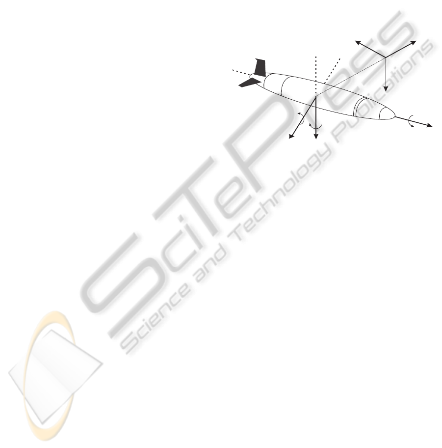
The AUV under study is a torpedo like underwater

vehicle and it is illustrated in Figure 1 with the rele-

vant body–ﬁxed and inertial coordinate systems. The

modeling of the equations of motion will be derived

by the utilization of a relative standard framework

that has been established in (Gertler and Hagen,

1967) and revised in (Humphreys, 1976) and (Feld-

man, 1979) with the assumptions: 1) the vehicle is

deeply submerged in a homogeneous and unbounded

liquid, 2) the vehicle does not experience memory

effects, 3) the simulator neglects the effects of the

vehicle passing through its own wake, and 4) the

vehicle does not experience underwater currents. In

addition, the following assumptions for the vehicle’s

dynamics are also necessary: 1) the vehicle is a rigid

body of constant mass, 2) the control ﬁns do not stall

regardless of angle of attack, and 3) the propulsion

model treats the vehicle propeller as a source of

constant thrust and torque. The vehicle equations

Sway

Pitch

Heave

Yaw

Surge

Roll

y θ,

z, ψ

x, φ

Body-Fixed

Coordinates

Earth-Fixed

Coordinates

Figure 1: Body Fixed and Inertial Coordinate System of the

AUV.

of motion in Figure 1, consist of the kinematics,

rigid-body and mechanic terms (Fossen, 1994a) and

by combining the equations for the vehicle rigid–

body dynamics with the equations for the forces and

the moments of the vehicle, we can conclude in the

following non–linear set of equations in a general

framework of six degrees of freedom plane. These

equations follow the SNAME convention (SNAME,

1950) for the assignment of the body–ﬁxed vehicle

coordinate system and are presented in the above for

retaining clarity.

Eq.1 - Surge:

(m− X

˙u

) ˙u+mz

˙q− my

˙r = X

+ X

u|u|

u|u| + (X

ωq

− m)ωq

+(X

+ mx

+ (X

υr

+ m)υr +(X

+ mx

−my

pq− mz

pr+ X prop (1)

Eq.2 - Sway:

(m−Y

)

υ+ mz

˙p− (mx

−Y

˙r

)˙r = Y

υ|υ|

υ|υ|+Y

r|r|

+ (Y

− m)ur + (Y

ωp

+ m)ωp+ (Y

− mx

)pq

uυ

uυ+ my

+ mz

qr+Y

uuδ

(2)

Eq.3 - Heave:

(m− Z

)

ω+ my

˙p− (mx

+ Z

˙q

) ˙q = Z

+ Z

ω|ω|

q|q|

q|q| + (Z

+ m)uq + (Z

υp

− m)υp+ (Z

− mx

)rp

uω

uω+ mz

+ q

) − my

rq+ Z

uuδ

(3)

A CONSTRAINED FINITE TIME OPTIMAL CONTROLLER FOR THE DIVING AND STEERING PROBLEM OF AN

AUTONOMOUS UNDERWATER VEHICLE

261

Eq.4 - Roll:

−mz

υ+ my

ω+ (I

− K

˙p

) ˙p = K

+ K

p|p|

−(I

− I

)qr + m(uq− υp) − mz

(ωp− ur) + K

prop

(4)

Eq.5 - Pitch:

˙u− (mx

+ M

)

ω+ (I

− M

˙q

) ˙q = M

+ M

ω|ω|

q|q|

q|q| + (M

− mx

)uq+ (M

υp

+ mx

)υp

+[M

− (I

− I

)]rp+ mz

(υr− ωq) + M

uω

uω+ M

uuδ

(5)

Eq.6 - Yaw:

−my

˙u+ (mx

+ N

)

υ+ (I

− N

˙r

)˙r = N

+ N

υ|υ|

r|r|

r|r| + (N

− mx

)ur + (N

ωp

+ mx

)ωp

+[N

− (I

− I

)]pq − my

(υr− ωq) + N

uυ

uυ+ N

uuδ

(6)

In these equations, the vehicle’s cross products of

inertia I

, I

were assumed to be small and ne-

glected. Moreover, zero value coefﬁcients have not

been included in the current formulation.

2.1 Diving Plane Motion

For deriving the equations of the diving plane motion,

we should take under consideration only the body–

relative surge velocity u, heave velocity ω, the pitch

rate q, the earth–relative vehicle forward position x,

the diving z, and the pitch angle θ. Before linearizing

these equations in (1-6) we will integrate the terms

for the hydrostatics, the axial and crossbow drag, the

added mass, the body and ﬁn lift and ﬁnally the mo-

ments. By assuming that the other velocities (υ, p,

r) are negligible, we can result in the following lin-

earized relationships between the body and earth ﬁxed

vehicle velocities (Prestero, 2001):

(m− X

˙u

) ˙u+ mz

˙q− X

u− X

q− X

θ = 0

(m− Z

)

ω− (mx

+ Z

˙q

) ˙q− Z

ω− (mU + Z

)q = Z

δs

˙u− (mx

+ M

)

ω+ (I

− M

˙q

) ˙q− M

ω+

(mx

U − M

)q− M

θ = M

(7)

where at this point and for clarity in our presentation,

the nomenclature that is ruling equations (1-7) is pre-

sented in Table 1.

If we assume that z

is small compared to the other

terms, we can decouple heave and pitch from surge,

which results in the following set of equations:

(m− Z

)

ω− (mx

+ Z

˙q

) ˙q− Z

ω− (mU + Z

)q = Z

δs (8)

−(mx

+ M

)

ω+ (I

− M

˙q

) ˙q− M

ω+

(mx

U − M

)q− M

θ = M

(9)

and based on the mentioned assumptions the vehicle’s

kinematic equations of motion are formulated as (Tri-

antafyllou and Franz, 2003):

Table 1: Utilized parameters and their values in the lin-

earized description of AUV’s diving motion.

Par. Name Par. Name

Center of gravity z

Center of gravity

Hydrostatic m AUV’s mass

Axial drag X

˙u

Added mass

Added mass I

Moment of inertia

˙q

Heave velocity U Steady velocity

Combined term Z

Added mass

Combined term Z

˙q

Added mass

Combined term M

Added mass

Combined term M

˙q

Added mass

Hydrostatic

˙x = cos(θ)u+ sin(θ)ω (10)

˙z = −sin(θ)u+ cos(θ)ω (11)

θ = q (12)

For the linearization of equations in (10-12) it is

assumed that the vehicle motion consists of small per-

turbationsaround a steady point. In this case,U repre-

sents the steady–state forward velocity of the vehicle.

If heave and pitch are linearized about zero, we have

u = U + u

′

, ω = ω

′

and q = q

′

. By utilizing: a) the

equations in (10–12), b) the Maclaurin expansion of

the trigonometric terms, c) dropping the higher order

terms, and d) with the above assumption for the de-

coupling of heave and pitch from surge, the following

linearized kinematic equations of motion are derived:

˙z = ω−Uθ (13)

θ = q (14)

The combination of equations (8) and (9) with

those in equations (13) and (14) results in the follow-

ing matrix form for the description of the diving plane

motion of the AUV:







m− X

˙u

−(mx

+ Z

˙q

) 0 0

−(mx

+ M

) I

− M

˙q

0 0

0 0 1 0

0 0 0 1













˙q

˙z







−







mU +Z

0 0

−mx

U + M

0 M

1 0 0 −U

0 1 0 0































[δ

] (15)

Assuming that the heave velocities are small com-

pared to the other terms, and that the center of gravity

is equal to the buoyancy center (x

= 0), the equations

in (15) are simpliﬁed to the following:







− M

˙q

0 0

0 1 0

0 0 1













˙q

˙z













−M

0 −M

0 0 U

−1 0 0































[δ

] (16)

ICINCO 2010 - 7th International Conference on Informatics in Control, Automation and Robotics

262

and ﬁnally for the state space description of the lin-

earized system, it is derived that:







˙q

˙z













−M

˙q

−M

˙q

0 0 −U

1 0 0

























−M

˙q







[δ

] (17)

Given the state vector x

= [q z θ]

′

∈ ℜ

and the input

con

= δ

∈ ℜ we can write the matrix form in (17) as:

˙x

= A

div

+ B

div

con

(18)

= C

div

(19)

with A

div







−M

˙q

−M

˙q

0 0 −U

1 0 0







, B

div







−M

˙q







and

div

= [1 0 0].

2.2 Steering Plane Motion

As it was presented in Section 2.2, the diving subsys-

tem controls depth and pitch errors while the steer-

ing subsystem controls heading errors. In the pre-

sented approach it is assumed that the upper–bow rud-

der and the lower–bow rudder, as also the upper–stern

and the lower–stern rudder of the AUV, are of iden-

tical size and shape and are receiving the deﬂection

command equally, at the same time instant, but in an

opposite direction. Moreover the following assump-

tions are made: 1) the center of mass of the vehicle

lies below the origin (z

is positive), 2) x

and y

are

zero, 3) the vehicle is symmetric in its inertial proper-

ties, 4) the motions in the vertical plane are negligible

([w

, p, q, r, Z, φ, θ] = 0), and 5) u

equals the forward

speed, U. Based on these assumptions and on the cal-

culation of the hydrodynamic coefﬁcients in (Fodrea,

2002), equations (1–6) are simpliﬁed to the following

linearized equations:

υ = −mUr+Y

υ+Y

˙r

˙r+Y

r+Y

(20)

˙r = N

υ+N

υ+ N

˙r

˙r+N

r+ N

(21)

ψ = r (22)

where the nomenclature that is ruling the above

set of equations is presented in Table 2.

Equations (20–21) in a matrix form could be writ-

ten as:







m−Y

−Y

˙r

−N

− N

˙r

0 0 1













˙r













− mU 0

0 1 0































[δ

] (23)

For the steering subsystem there are three state

variables: r, ψ, ad υ. The r variable is the yaw rate of

turn, ψ variable represents the heading angle, while υ

Table 2: Utilized parameters and their values in the lin-

earized description of AUV’s Steering motion.

Par. Name

Added mass is sway

˙r

Added mass in yaw

Sway force induced by side slip

Sway force induced by yaw

Added mass in sway

˙r

Added mass in yaw

Sway moment from side slip

Sway moment from yaw

Linearized rudder action force

represents the sway velocity. Based on the assump-

tion made for the vehicle dynamics is that the cross

coupling terms in the mass matrix are zero due to the

assumed symmetry in the rudders, equation (23) can

be given as:







m−Y

0 0

0 I

− N

˙r

0 0 1













˙r













− mU 0

0 1 0































[δ

] (24)

where δ

is the control signal applied to both rudders.

The state space description of the linearized system

will be:







˙r













m−Y

−mU

m−Y

−N

˙r

−N

˙r

0 1 0

























m−Y

−N

˙r







[δ

] (25)

Given the state vector x

= [υ r ψ]

′

∈ ℜ

and the

input u

con

= δ

∈ ℜ, the matrix form in Eq. (25) can

be written as:

˙x

= A

steer

+ B

steer

con

(26)

= C

steer

(27)

where

steer







m−Y

−mU

m−Y

−N

˙r

−N

˙r

0 1 0







, B

steer







m−Y

−N

˙r







and

steer

1 0 0

3 CONSTRAINED FINITE TIME

OPTIMAL CONTROLLER

SYNTHESIS

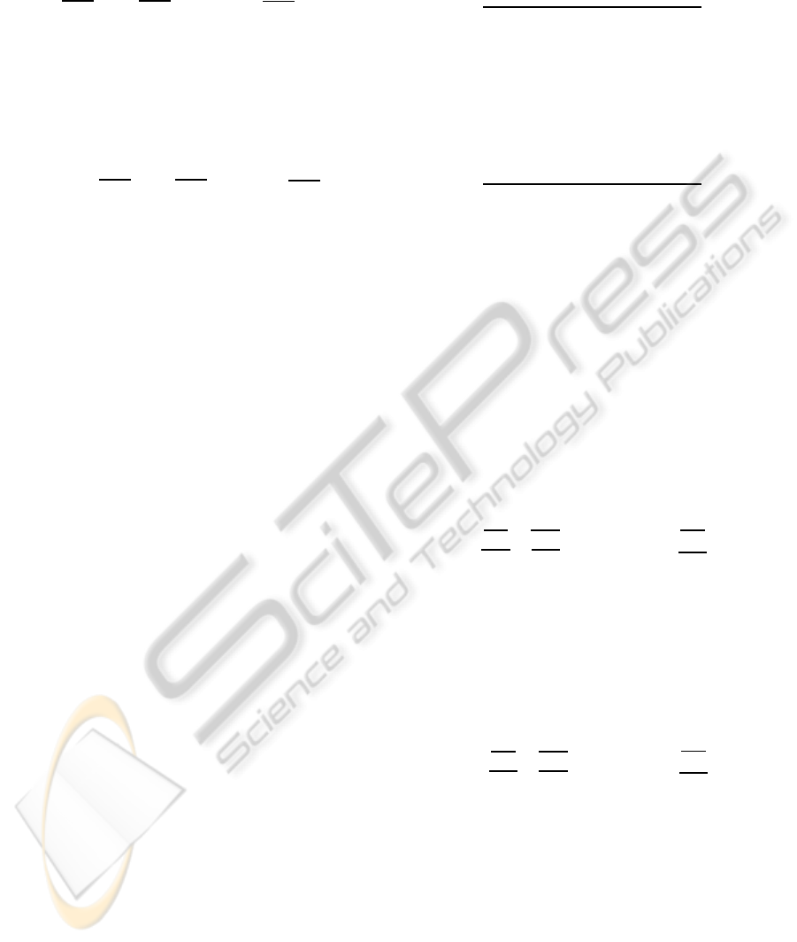
In the proposed control strategy, the aim is to design

a CFTOC–scheme for the decoupled diving and steer-

ing motion of the AUV as it is presented in Figure 2.

At this point it should be mentioned that the speed

A CONSTRAINED FINITE TIME OPTIMAL CONTROLLER FOR THE DIVING AND STEERING PROBLEM OF AN

AUTONOMOUS UNDERWATER VEHICLE

263

u ∈ ℜ of the AUV was considered to be constant and

no control action has been considered for this mo-

tion while the control actions are applied to the lin-

ear model of the AUV after the ZOH. Prior to the de-

sign of the control algorithm, it is necessary to model

and take under consideration in the controller’s syn-

thesis, the mechanical constrains of the utilized AUV,

the disturbances that are introduced from the onboard

sensors, the additive uncertainties due to modeling er-

rors and the non–linearities.

AUV

Model

CFTO

Controller

ZOH

Sampler

Reference

Figure 2: The Proposed Control Scheme for the AUV’s

Depth and Steering Motions

The derived linearized decoupled models in equa-

tions (18-19) and (26-27) are valid only for small val-

ues of pitch, yaw and ﬁn angles around the lineariza-

tion points. Moreover, the control actions u

con

, u

con

should also be bounded due to physical constraints

applied to the motors. We consider the state vec-

tor X = [x

, x

]

∈ ℜ

and the control vector U =

con

, u

con

]

∈ ℜ

Let the matrix H

be a zeroed 2 × 8 matrix except

for its i–th column, which is equal to [1, −1]

and

with i ∈ [1, 2, ·· · , 16], i.e.:



0 ... 0 1 0 ... 0

0 ... 0 −1 0 ... 0



(28)

The bounds can be cast in a more compact form as:







−−







16×8





−−





8×1

≤







max

min

max

min

−−

max

min

max

min







16×1

(29)

where the notation X

corresponds to the ith element

of the vector X .

Due to factors such as noise, accuracy of measure-

ments and round–off errors, the onboard measure-

ments are not ideal. These inaccuracies in the mea-

surements, in the presented approach are considered

as additive disturbances to the system models. More-

over we will consider uncertainty in the state space

matrices, due to the existence of modelling simpliﬁ-

cations and errors. If we consider a sampling time

∈ ℜ

, the combined discrete time version of equa-

tions (18-19) and (26-27) with the effects of the ad-

ditive noise, can be cast as piecewise afﬁne (PWA)

system:

X =

∗,i

div

3×3

∗,i

steer

X +

∗,i

div

∗,i

steer

U +W (30)

with the constraints in (29). The notation (·)

∗

repre-

sents the discrete time value of the corresponding ma-

trix, while W ∈ ℜ

is an additive and of a zero mean

white noise, bounded by the set W ⊆ ℜ

. Moreover

j ∈ S , with S , {1, 2, · · · , s}, is a ﬁnite set of indexes

and s ∈ Z

denotes the number of afﬁne sub–systems

in (30). For polytopic uncertainty, Ω is the polytope

deﬁned as:

Ω = Co{[A

∗,1

div

∗,1

steer

∗,1

div

∗,1

steer

], ··· , [A

∗,s

div

∗,s

steer

∗,s

div

∗,s

steer

]}, (31)

where Co denotes the convex hull and

∗,i

div

∗,i

steer

∗,i

div

∗,i

steer

] are vertices of the con-

vex hull. Any [A

∗

div

∗

steer

∗

div

∗

steer

] within the

convex set Ω is a linear combination of the vertices:

∗

div

∗

steer

∗

div

∗

steer

] =

∑

j=1

∗

div

∗

steer

∗

div

∗

steer

] (32)

with

∑

j=1

= 1, 0 ≤ a

≤ 1.

The CFTOC-design problem consists of com-

puting the optimum control vector sequence

U =

k+1

... U

k+N−1

]

, where N corresponds to the

prediction horizon that minimizes the following cost

function:

, X

) = [X

k+N

− X

)]

P[X

k+N

− X

] +

N−1

∑

m=0

k+m

]

R[U

k+m

] + [X

k+m

− X

]

Q[X

k+m

− X

]

where

P ∈ ℜ

6×6

with

P =

≥ 0, R ∈ ℜ

2×2

with

R = R

> 0 and Q ∈ ℜ

6×6

with Q = Q

≥ 0, are full

column rank weighting matrices penalizing the corre-

sponding optimization variables i.e predicted states,

control effort and the desired ﬁnal state, respectively,

while X

is the reference set–point.

The solution to the CFTOC problem (Borelli et al.,

2003; Grieder et al., 2004; Kvasnica et al., 2004) is a

continuous control action of the form:

= F

+ G

if X

∈

(33)

where

, l ∈ {1, ...l

max

} corresponds to a convex

polyhedron (

∈ ℜ

) calculated by the algorithm,

ICINCO 2010 - 7th International Conference on Informatics in Control, Automation and Robotics

264

and F

∈ ℜ

2×6

, G

∈ ℜ

2,1

. The l

max

–number of poly-

hedra is similarly speciﬁed by the algorithm. In gen-

eral the higher the number of the PWA–systems along

with the large dimension of the state vector and the

number of constraints, the more complicated the so-

lution is.

This complexity increases signiﬁcantly with the

value of the prediction horizon N, and the number

max

of the convex polyhedra (regions) grows up (usu-

ally) exponentially. Certain techniques have been de-

vised to merge the various regions into larger ones

without signiﬁcantly compromising the validity of the

solution. For the on–line implementation of the con-

troller the number l

max

of the regions is not only a

measure of the controller’s complexity but also affects

its implementation typically precomputed in a look–

up table.

4 SIMULATION STUDIES

The proposed CFTO–control scheme has been ap-

plied in simulation studies on the model of the RE-

MUS AUV. Based on experimental results in (Pres-

tero, 2000) the parameters presented in Tables I and

II were tuned and the continuous time state space ma-

trices for the diving and steering motion of the AUV

are:

div







−0.82 0 −0.69

0 0 −1.54

1 0 0







, B

div







−4.16







(34)

steer







−1.01 −0.68 0

−0.54 −0.82 0

0 1 0







, B

steer







0.22

−1.19







(35)

The constraints on the control inputs and the out-

puts have been arbitrary set to: u

con

min

= −10 ≤

con

(t) ≤ 10 = u

con

max

, u

con

min

= −60 ≤ u

con

(t) ≤

60 = u

con

max

and y

min

= −50

≤ y

(t) ≤ 50

= y

max

min

= −70

≤ y

(t) ≤ 50

= y

max

respectively. The

constrains for the states have been set as:

−30

≤ X

≤ 30

−20

≤ X

≤ 20

−360 ≤ X

≤ −360

−50

≤ X

≤ 50

−40

≤ X

≤ 40

−360 ≤ X

≤ −360

For the state space matrices

div

, B

div

, A

steer

, B

steer

, we assume that there is

an additive corrupting uncertainty of 1%, while the

additive disturbances have been set to 0.01 · I

6×1

The selection that has been made on the penalizing

matrices for the CFTOC cost was P = 10

· I

6×6

R = I

2×2

and Q = 10

· I

6×6

. The output set–point

was selected for the diving motion as Y

ref

= 5

and Y

ref

= 5

for the steering motion. The initial

augmented state vector was X

init

= O

6×1

. For the

controllers formulation the 2− vector norm case was

tested and the discretization has been made with a

sampling period of T

= 1sec.

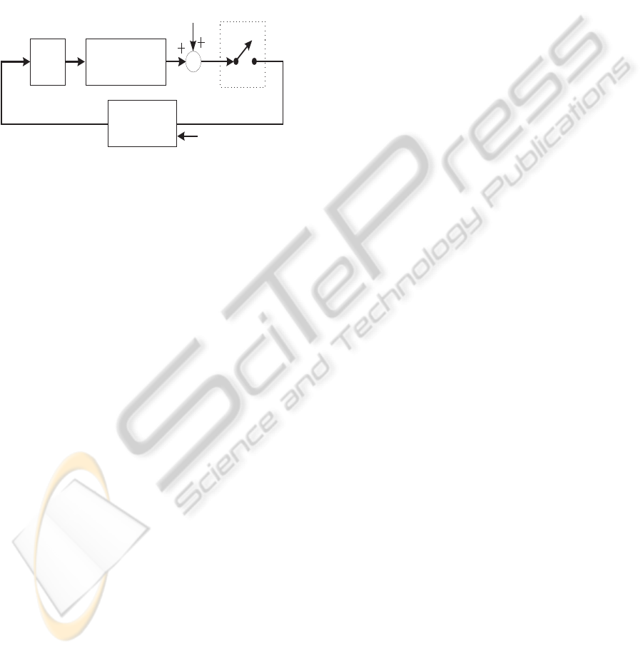
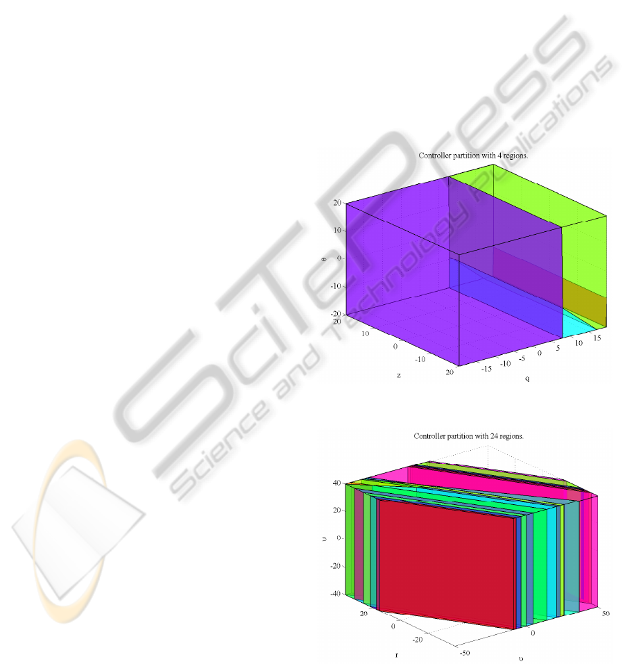
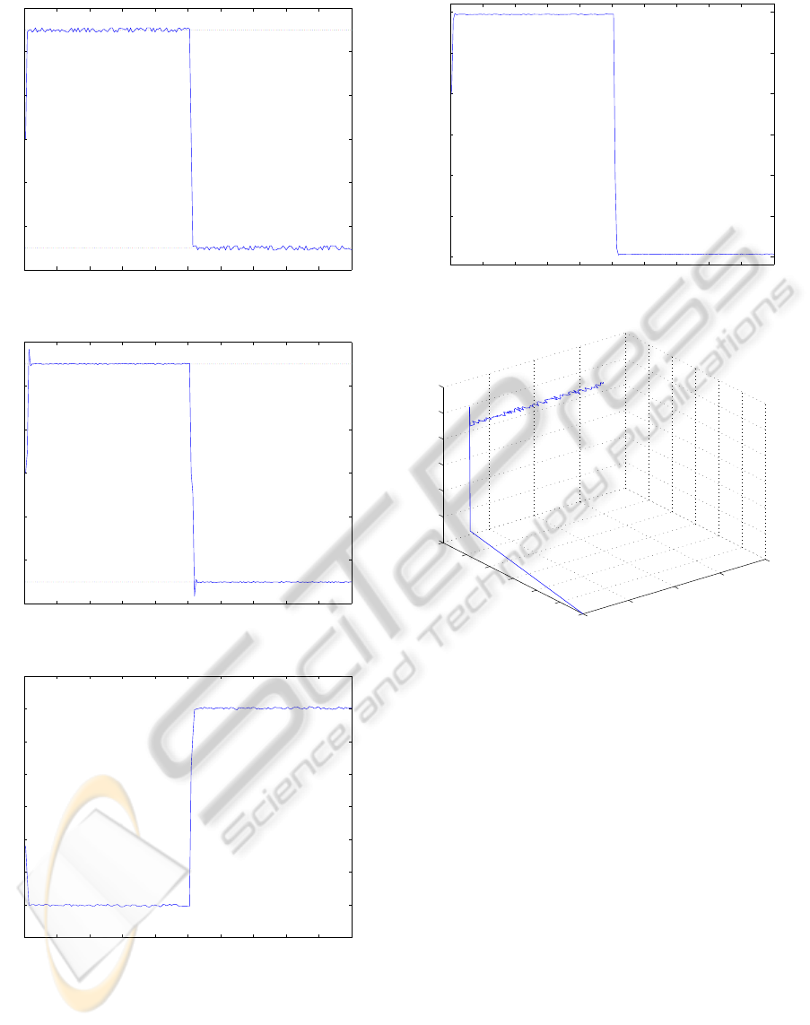
The resulting controllers’ partitions for the diving

and steering motion are presented in Figures 3 and 4,

while the responses of the diving and steering motions

are displayed in Figures 5 and 6 respectively, while

the controllers’ response for the cases of the diving

and steering motion are presented in Figures 7 and 8

respectively. Finally in Figure 9 the 3–D combined

movement of the AUV (including displacement with

a constant speed (U=1.54m/sec) is displayed.

Figure 3: CFTO–Controller Partitioning for the Diving Mo-

tion.

Figure 4: CFTO–Controller Partitioning for the Steering

Motion.

A CONSTRAINED FINITE TIME OPTIMAL CONTROLLER FOR THE DIVING AND STEERING PROBLEM OF AN

AUTONOMOUS UNDERWATER VEHICLE

265

0 20 40 60 80 100 120 140 160 180 200

−6

−4

−2

Time(sec)

Diving Motion (Deg)

Figure 5: Diving Motion Time Response.

0 20 40 60 80 100 120 140 160 180 200

−6

−4

−2

Time(sec)

Steering Motion (Deg)

Figure 6: Steering Motion Time Response.

0 20 40 60 80 100 120 140 160 180 200

−4

−3

−2

−1

Time(sec)

Control Effort for the Diving Motion

Figure 7: Controller Effort for the Diving Motion.

5 CONCLUSIONS

In this paper a constrained ﬁnite time optimal con-

troller for the diving and steering motion of an AUV

has been presented. The utilized proposed scheme

0 20 40 60 80 100 120 140 160 180 200

−15

−10

−5

Time(sec)

Control Effort for the Steering Motion

Figure 8: Controller Effort for the Steering Motion.

100

150

200

Figure 9: 3–D Combined movement of the AUV.

was developed based on the decoupled equations of

motion for the diving and steering of the AUV. The

derived Constrained Finite Time Optimal control had

the ability to take under consideration: a) the con-

strains on the inputs, outputs, and the states of the

model, b) the corrupting disturbances due to the ex-

istence of the noise in the measurements, and c) the

uncertainty in the modeling procedures. Simulation

results have been presented that prove the validity of

the proposed scheme.

REFERENCES

Bjorn, J. (1994). The NDRE-AUV Flight Control System.

IEEE journal of Oceanic Engineering, 19(4).

Borelli, F., Baotic, M., Bemporad, A., and Morari, M.

(2003). An Efﬁcient Algorithm for Computing the

State Feedback Optimal Control Law for Discrete

Time Hybrid Systems.

Cristi, R., Papoulias, A., and Healey, A. J. (1990). Adap-

ICINCO 2010 - 7th International Conference on Informatics in Control, Automation and Robotics

266

tive Sliding Mode Control of Autonomous Undewater

Vehicle in the Dive Plane. IEEE Journal of Oceanic

Engineering, 15(3).

Debitetto, A. (1995). Fuzzy logic for depth control of un-

manned undersea vehicles. IEEE journal of Oceanic

Engineering, 20(3).

E. An, R. Dhanak, L. S. S. S. J. L. (2001). Coastal oceanog-

raphy using a small auv. Journal of Atmospheric and

Ocean Technology, (18):215–234.

Feldman, J. (1979). Revised standard submarine equations

of motion report dtnsrdc/spd-0393-09. Technical re-

port, David W. Taylor Naval Ship Research and De-

velopment Center, Bethesda, MD.

Field, A. I. (2000). Optimal control of an autonomous un-

derwater vehicle. In World Automatic Congress, Maui,

Hawaii.

Fodrea, L. R. (2002). Obstactle Avoidance Control for the

REMUS Autonomous Underwater Vehicle. PhD the-

sis, Naval Postgraduate School, Monterey, California.

Foresti, G. (2001). Visual inspection of sea bottom struc-

tures by an autonomous underwater vehicle. IEEE

Transactions on Systems, Man and Cybernetics - Part

B: cybernetics, 31(5).

Fossen, T. (1994a). Guidance and control of ocean vehicles.

John Wiley & Sons Ltd.

Fossen, T. I. (1994b). Guidance and Control of an Au-

tonomous Underwater Vehicle. John Wiley and Sons.

Gertler, M. and Hagen, G. (1967). Standard equations of

motion for submarine simulation report dtnsrdc 2510.

Technical report, David W. Taylor Naval Ship Re-

search and Development Center, Bethesda.

Grieder, P., Borelli, F., Torrisi, F., and Morari, M. (2004).

Computation of the Constrained Inﬁnite Time Linear

Quadratic Regulator. Automatica, 40(4):701–708.

Healey, A. and Lienard, D. (1993). Multivariable sliding

mode control for autonomous diving and steering of

unmanned underwater vehicles. In IEEE Journal of

Oceanic Engineering, volume 18.

Humphreys, D. (1976). Development of the equations of

motion and transfer functions for underwater vehicles.

Technical report, Naval Coastal Systems Laboratory,

Panama City, FL.

Kawano, H. and Ura, T. (2002). Fast reinforcement learn-

ing algorithm for motion planning of non-holonomic

unmanned underwater vehicles. In Int. Conference on

Intelligent Robots and Systems IEEE/RSJ, Lausanne,

Switzerland.

Kvasnica, M., Grieder, P., Baotic, M., and Morari, M.

(2004). Multi–Parametric Toolbox (MPT). Hybrid

Systems: Computation and Control, (2993):448–462.

Pestero, T. (2001). Veriﬁcation of six–degree of freedom

simulation model for the remus auv. Master’s thesis,

Massachusetts Institute of Technology.

Prestero, T. (2000). Development of a six–degree of free-

dom simulation model for the remus autonomous un-

derwater vahicle. In In Proceedings of MTS-IEEE

Oceans 2000,Providence, Rhode Island.

Prestero, T. (2001). Veriﬁcation of a six-degree of freedom

simulation model for the remus autonomous underwa-

ter vehicle. Master’s thesis, Massachusetts Institute of

Technology and Woods Hole Oceanographic Institu-

tion, Cambridge, Massachusetts.

Rodrigues, L., Tavares, P., and Prado, M. (1996). Slid-

ing mode control of an auv in the diving and steering

planes. In OCEANS MTS/IEEE.

SNAME (1950). Nomenclature for treating the motion of a

submerged body through a ﬂuid. The Society of Naval

Architects and Marine Engineers, Technical and Re-

serach Bulletin, (1-5):1–15.

Triantafyllou, M. and Franz, S. (2003). Hover maneuvering

and control of marine vehicles. Lectures.

Yuh, J. (2000). Design and control of autonomous underwa-

ter robots: A survey. Autonomous Robots, 8(1):7–24.

A CONSTRAINED FINITE TIME OPTIMAL CONTROLLER FOR THE DIVING AND STEERING PROBLEM OF AN

AUTONOMOUS UNDERWATER VEHICLE

267