ROBUSTNESS OF ISS SYSTEMS TO INPUTS WITH LIMITED

MOVING AVERAGE, WITH APPLICATION TO SPACECRAFT

FORMATIONS

Esten Ingar Grøtli

, Antoine Chaillet

, Elena Panteley

and Jan Tommy Gravdahl

Dept. of Eng. Cybernetics, NTNU, O. S. Bragstads plass 2D, 7491 Trondheim, Norway

Univ. Paris Sud 11 - L2S - EECI - Sup

elec, 3 rue Joliot-Curie, 91192 Gif Sur Yvette, France

CNRS - L2S, Sup

elec, 3 rue Joliot-Curie, 91192 Gif Sur Yvette, France

Keywords:

Robustness, ISS, Moving average of disturbances, Spacecraft formation.

Abstract:

We provide a theoretical framework that ﬁts realistic challenges related to spacecraft formation with distur-

bances. We show that the input-to-state stability of such systems guarantees some robustness with respect to

a class of signals with bounded average-energy, which encompasses the typical disturbances acting on space-

craft formations. Solutions are shown to converge to the desired formation, up to an offset which is somewhat

proportional to the considered moving average of disturbances. The approach provides a tighter evaluation of

the disturbances’ inﬂuence, which allows for the use of more parsimonious control gains.

1 INTRODUCTION

Spacecraft formation control is a relatively new and

active ﬁeld of research. Formations, characterized

by the ability to maintain relative positions without

real-time ground commands, are motivated by the aim

of placing measuring equipment further apart than

what is possible on a single spacecraft. This is de-

sirable as the resolution of measurements often are

proportional to the baseline length, meaning that ei-

ther a large monolithic spacecraft or a formation of

smaller, but accurately controlled spacecraft, may be

used. Monolithic spacecraft architecture that satisfy

the demand of resolution are often both impractical

and costly to develop and to launch. On the other

hand, smaller spacecrafts may be standardized and

have lower development cost. In addition they may

be of a lower collective weight and/or of smaller col-

lective size such that cheaper launch vehicles can be

used. There is also the possibility for them to piggy-

back with other commercial spacecraft. These advan-

tages, come at the cost of an increased complexity.

From a control design perspective, a crucial challenge

is to maintain a predeﬁned relative trajectory, even in

presence of disturbances. Most of these disturbances

are hard to model in a precise manner. Only statistical

or averaged characteristics of the perturbing signals

(e.g. amplitude, energy, average energy, etc.) are typ-

ically available. These perturbing signals may have

diverse origins:

• Intervehicle Interference. In close formation or

spacecraft rendezvous, thruster ﬁrings and ex-

haust gases may inﬂuence other spacecraft.

• Solar wind and Radiation. Particles and radiation

expelled from the sun inﬂuence the spacecraft and

are highly dependent on the solar activity (Wertz,

1978), which is difﬁcult to predict (Hanslmeier

et al., 1999).

• Small Debris. While large debris would typically

mean the end of the mission, some space trash, in-

cluding paint ﬂakes, dust, coolant and even small

needles

, is small enough to “only” deteriorate the

performance, see (NASA, 1999).

• Micrometeroids. The damages caused by microm-

eteroids may be limited due to their tiny size, but

constant high velocity impacts also degrade the

performance of the spacecraft through momentum

transfer (Sch

afer, 2006).

• Gravitational Disturbances. Even gravitational

Project West Ford was a test carried out in the early

1960s, where 480 million needles were placed in orbit, with

the aim to create an artiﬁcial ionosphere above the Earth to

allow global radio communication, (Overhage and Radford,

1964).

Ingar Grøtlia E., Chaillet A., Panteley E. and Tommy Gravdahl J. (2010).

ROBUSTNESS OF ISS SYSTEMS TO INPUTS WITH LIMITED MOVING AVERAGE, WITH APPLICATION TO SPACECRAFT FORMATIONS.

In Proceedings of the 7th International Conference on Informatics in Control, Automation and Robotics, pages 35-44

DOI: 10.5220/0002946500350044

 SciTePress

models including higher order zonal harmonics,

can only achieve a limited level of accuracy due

to the shape and inhomogeneity of the Earth. In

addition comes the gravitational perturbation due

to other gravitating bodies such as the Sun and the

Moon.

• Actuator Mismatch. There will commonly be a

mismatch between the actuation computed by the

control algorithm, and the actual actuation that the

thrusters can provide. This mismatch is particu-

larly present if the control algorithm is based on

continuous dynamics, without taking into account

pulse based thrusters.

Nonlinear control theory provides instruments to

guarantee a prescribed precision in spite of these dis-

turbances. Input-to-state stability (ISS) is a con-

cept introduced in (Sontag, 1989), which has been

thoroughly treated in the literature: see for instance

the survey (Sontag, 2008) and references therein.

Roughly speaking, this robustness property ensures

asymptotic stability, up to a term that is “propor-

tional” to the amplitude of the disturbing signal. Simi-

larly, its integral extension, iISS (Sontag, 1998), links

the convergence of the state to a measure of the energy

that is fed by the disturbance into the system. How-

ever, in the original works on ISS and iISS, both these

notions require that these indicators (amplitude or en-

ergy) be ﬁnite to guarantee some robustness. In par-

ticular, while this concept has proved useful in many

control application, ISS may yield very conservative

estimates when the disturbing signals come with high

amplitude even if their moving average is reasonable.

These limitations have already been pointed out

and partially addressed in the literature. In (Angeli

and Ne

c, 2001), the notions of “Power ISS” and

“Power iISS” are introduced to estimate more tightly

the inﬂuence of the power or moving average of the

exogenous input on the power of the state. Under the

assumption of local stability for the zero-input sys-

tem, these properties are shown to be actually equiv-

alent to ISS and iISS respectively. Nonetheless, for a

generic class of input signals, no hard bound on the

state norm can be derived for this work.

Other works have focused on quantitative aspects

of ISS, such as (Praly and Wang, 1996), (Gr

une,

2002) and (Gr

une, 2004). All these three papers solve

the problem by introducing a “memory fading” effect

in the input term of the ISS formulation. In (Praly and

Wang, 1996) the perturbation is ﬁrst fed into a linear

scalar system whose output then enters the right hand

side of the ISS estimate. The resulting property is re-

ferred to as exp-ISS and is shown to be equivalent to

ISS. In (Gr

une, 2002) and (Gr

une, 2004) the concept

of input-to-state dynamical stability (ISDS) is intro-

duced and exploited. In the ISDS state estimate, the

value of the perturbation at each time instant is used

as the initial value of a one-dimensional system, thus

generalizing the original idea of Praly and Wang. The

quantitative knowledge of how past values of the in-

put signal inﬂuence the system allows, in particular, to

guarantee an explicit decay rate of the state for van-

ishing perturbations.

In this paper, our objective is to guarantee hard

bound on the state norm for ISS systems in presence

of signals with possibly unbounded amplitude and/or

energy. We enlarge the class of signals to which ISS

systems are robust, by simply conducting a tighter

analysis on these systems. In the spirit of (Angeli

and Ne

c, 2001), and in contrast to most previous

works on ISS and iISS, the considered class of dis-

turbances is deﬁned based on their moving average.

We show that any ISS system is robust to such a class

of perturbations. When an explicitly Lyapunov func-

tion is known, we explicitly estimate the maximum

disturbances’ moving average that can be tolerated

for a given precision. These results are presented in

Section 2. We then apply this new analysis result

to the control of spacecraft formations. To this end,

we exploit the Lyapunov function available for such

systems to identify the class of signals to which the

formation is robust. This class includes all kind of

perturbing effects described above. This study is de-

tailed, and illustrated by simulations, in Section 3.

Notation and Terminology

A continuous function α : R

≥

→ R

≥0

is of class K

(α ∈ K ), if it is strictly increasing and α(0) = 0. If,

in addition, α(s) → ∞ as s →∞, then α is of class K

∞

(α ∈ K

∞

). A continuous function β : R

≥0

×R

≥0

→

≥0

is said to be of class K L if, β(·,t) ∈ K for any

t ∈ R

≥0

, and β(s,·) is decreasing and tends to zero

as s tends to inﬁnity. The solutions of the differential

equation ˙x = f (x, u) with initial condition x

∈ R

denoted by x(·; x

,u). We use |·| for the Euclidean

norm of vectors and the induced norm of matrices.

The closed ball in R

of radius δ centered at the ori-

gin is denoted by B

, i.e. B

:= {x ∈ R

: |x| ≤ δ}.

|·|

denotes the distance to the ball B

, that is |x|

inf

z∈B

|x −z|. U denotes the set of all measurable lo-

cally essentially bounded signals u : R

≥0

→ R

. For

a signal u ∈ U, kuk

∞

:= ess sup

t≥0

|u(t)|. The maxi-

mum and minimum eigenvalue of a symmetric matrix

A is denoted by λ

max

(A) and λ

min

(A), respectively. I

and 0

denote the identity and null matrices of R

n×n

respectively.

ICINCO 2010 - 7th International Conference on Informatics in Control, Automation and Robotics

2 ISS SYSTEMS AND SIGNALS

WITH LOW MOVING

AVERAGE

2.1 Preliminaries

We start by recalling some classical deﬁnitions related

to the stability and robustness of nonlinear systems of

the form

˙x = f (x,u), (1)

where x ∈ R

, u ∈ U and f : R

×R

→R

is locally

Lipschitz and satisﬁes f (0, 0) = 0.

Deﬁnition 1. Let δ be a positive constant and u be a

given signal in U. The ball B

is said to be globally

asymptotically stable (GAS) for (1) if there exists a

class K L function β such that the solution of (1) from

any initial state x

∈ R

satisﬁes

|x(t;x

,u)| ≤ δ +β(|x

|,t), ∀t ≥ 0. (2)

Deﬁnition 2. The ball B

is said to be globally ex-

ponentially stable (GES) for (1) if the conditions of

Deﬁnition 1 hold with β(r,s) = k

−k

for some pos-

itive constants k

and k

We next recall the deﬁnition of ISS, originally in-

troduced in (Sontag, 1989).

Deﬁnition 3. The system ˙x = f (x, u) is said to be

input-to-state stable (ISS) if there exist β ∈ K L and

γ ∈ K

∞

such that, for all x

∈ R

and all u ∈ U, the

solution of (1) satisﬁes

|x(t;x

,u)| ≤ β(|x

|,t) +γ(kuk

∞

), ∀t ≥ 0 . (3)

ISS thus imposes an asymptotic decay of the norm

of the state up to a function of the amplitude kuk

∞

the input signal.

We also recall the following well-known Lya-

punov characterization of ISS, originally established

in (Praly and Wang, 1996) and thus extending the

original characterization proposed by Sontag in (Son-

tag and Wang, 1995).

Proposition 1. The system (1) is ISS if and only if

there exist α, α,γ ∈ K

∞

and κ > 0 such that, for all

x ∈R

and all u ∈ R

α(|x|) ≤V (x) ≤ α(|x|) (4)

∂V

∂x

(x) f (x,u) ≤ −κV (x)+ γ(|u|) . (5)

γ is then called a supply rate for (1).

Remark 1. Since ISS implies iISS (cf. (Sontag,

1998)), it can be shown that the solutions of any ISS

system with supply rate γ satisﬁes, for all x

∈ R

|x(t;x

,u)|≤β(|x

|,t)+η



γ(|u(τ)|)dτ



, ∀t ≥0 ,

(6)

where β ∈ K L and η ∈ K

∞

. The above integral can

be seen as a measure, through the function γ, of the

energy of the input signal u.

The above remark establishes a link between a

measure of the energy fed into the system and the

norm of the state: for ISS (and iISS) systems, if this

input energy is small, then the state will eventually be

small. However, Inequalities (3) and (6) do not pro-

vide any information on the behavior of the system

when the amplitude (for (3)) and/or the energy (for

(6)) of the input signal is not ﬁnite.

From an applicative viewpoint, the precision guar-

anteed by (3) and (6) involve the maximum value and

the total energy of the input. These estimates may

be conservative and thus lead to the design of greedy

control laws, with negative consequences on the en-

ergy consumption and actuators solicitation. This is-

sue is particularly relevant for spacecraft formations

in view of the inherent fuel limitation and limited

power of the thrusters.

(Angeli and Ne

c, 2001) has started to tackle this

problem by introducing ISS and iISS-like properties

for input signals with limited power, thus not neces-

sarily bounded in amplitude nor in energy. For sys-

tems that are stable when no input is applied, the

authors show that ISS (resp. iISS) is equivalent to

“power ISS” (resp. “power iISS”) and “moving av-

erage ISS” (resp. “moving average iISS”). In general

terms, these properties evaluate the inﬂuence of the

amplitude (resp. the energy) of the input signal on the

power or moving average of the state. However, as

stressed by the authors themselves, these estimates do

not guarantee in general any hard bound on the state

norm. Here, we consider a slightly more restrictive

class of input signals under which such a hard bound

can be guaranteed. Namely, we consider input signals

with bounded moving average.

Deﬁnition 4. Given some constants E, T > 0 and

some function γ ∈ K , the set W

(E, T ) denotes the

set of all signals u ∈ U satisfying

t+T

γ(|u(s)|)ds ≤ E , ∀t ∈ R

≥0

The main concern here is the measure E of the

maximum energy that can be fed into the system over

a moving time window of given length T . These

quantities are the only information on the distur-

bances that will be taken into account in the control

design. More parsimonious control laws than those

based on their amplitude or energy can therefore be

expected. We stress that signals of this class are not

necessarily globally essentially bounded, nor are they

required to have a ﬁnite energy, as illustrated by the

following examples. Robustness to this class of sig-

ROBUSTNESS OF ISS SYSTEMS TO INPUTS WITH LIMITED MOVING AVERAGE, WITH APPLICATION TO

SPACECRAFT FORMATIONS

0 1 2 3 4 5 6 7 8 9

u(t)

Figure 1: An example of unbounded signal with bounded

moving average.

nals thus constitutes an extension of the typical prop-

erties of ISS systems.

Example 1.

1. Unbounded signals: given any T > 0 and any γ ∈

K , the following signal belongs to W

(1,T ) and

satisﬁes limsup

t→∞

|u(t)| = +∞:

u(t) :=



2k if t ∈ [2kT ;2kT +

], k ∈ N

0 otherwise.

The signal for T = 1 is illustrated in Figure 1.

2. Essentially bounded signals: given any T > 0 and

any γ ∈ K , if kuk

∞

is ﬁnite then it holds that

u ∈W

(T γ(kuk

∞

),T ). We stress that this includes

signals with inﬁnite energy (think for instance of

constant non-zero signals).

2.2 Robustness of ISS Systems to

Signals in the Class W

The following result establishes that the impact of an

exogenous signal on the qualitative behavior of an ISS

systems is negligible if the moving average of this sig-

nal is sufﬁciently low.

Theorem 1. Assume that the system ˙x = f (x,u) is ISS.

Then there exists a function γ ∈ K

∞

and, given any

precision δ > 0 and any time window T > 0, there

exists a positive average energy E(T,δ) such that the

ball B

is GAS for any u ∈ W

(E, T ).

The above result, proved in Section 4, adds an-

other brick in the wall of nice properties induced by

ISS, cf. (Sontag, 2008) and references therein. It en-

sures that, provided that a steady-state error δ can be

tolerated, every ISS system is robust to a class of dis-

turbances with sufﬁciently small moving average.

If an ISS Lyapunov function is known for the sys-

tem, then an explicit bound on the tolerable average

excitation can be provided based on the prooﬂines of

Theorem 1. More precisely, we state the following

result.

Corollary 1. Assume there exists a continuously dif-

ferentiable function V : R

→R

≥0

, class K

∞

functions

γ, α and α and a positive constant κ such that (4) and

(5) hold for all x ∈ R

and all u ∈ R

. Given any pre-

cision δ > 0 and any time window T > 0, let E denote

any average energy satisfying

E(T, δ) ≤

α(δ)

κT

−1

κT

−1

. (7)

Then the ball B

is GAS for ˙x = f (x, u) for any u ∈

(E, T ).

The above statement shows that, by knowing a

Lyapunov function associated to the ISS of a system,

and in particular its dissipation rate γ, one is able to

explicitly identify the class W

(E, T ) to which it is

robust up to the prescribed precision δ.

In a similar way, we can state sufﬁcient condition

for global exponential stability of some neighborhood

of the origin. This result follows also trivially from

the proof of Theorem 1.

Corollary 2. If the conditions of Corollary 1 are sat-

isﬁed with α(s) = cs

and α(s) = cs

, with c, c, p pos-

itive constants, then, given any T,δ > 0, the ball B

is GES for (1) with any signal u ∈W

(E, T ) provided

that

E(T, δ) ≤

cδ

κT

−1

κT

−1

3 ILLUSTRATION: SPACECRAFT

FORMATION CONTROL

We now exploit the results developed in Section 2 to

demonstrate the robustness of a spacecraft formation

control in a leader-follower conﬁguration, when only

position is measured. The focus on output feedback in

this illustration is motivated by the fact that velocity

measurements in space may not be easily achieved,

e.g. because the spacecraft cannot be equipped with

the necessary sensors for such measurements due to

space constraints or budget limits. The models de-

scribed in this section have strong resemblance with

the model of a robot manipulator. Our control de-

sign is therefore be based on control algorithms al-

ready validated for robot manipulators, in particular

(Berghuis and Nijmeijer, 1993) and (Paden and Panja,

1988). We stress that he proposed study is made for

two spacecraft only, but can easily be extended to for-

mations involving more spacecrafts.

ICINCO 2010 - 7th International Conference on Informatics in Control, Automation and Robotics

3.1 Spacecraft Models

The spacecraft models presented in this section are

similar to the ones derived in (Ploen et al., 2004).

All coordinates, both for the leader and the follower

spacecraft, are expressed in an orbital frame, which

origin relative to the center of Earth is given by ~r

and satisﬁes Newton’s gravitational law

= −

µ being the gravitational constant of Earth. The unit

vectors are such that ~o

:=~r

/|~r

| points in the anti-

nadir direction, ~o

:= (~r

)/|~r

| points in the

direction of the orbit normal, and ﬁnally ~o

:= ~o

completes the right-handed orthogonal frame. We

let ν

denote the true-anomaly of this reference frame

and assume the following:

Assumption 1. The true anomaly rate

and true

anomaly rate-of-change

of the reference frame sat-

isfy k

∞

≤ β

and k

∞

≤ β

, for some positive

constants β

and β

Note that this assumption is naturally satisﬁed

when the reference frame is following a Keplerian or-

bit, but it also holds for any sufﬁciently smooth refer-

ence trajectory. We deﬁne the following quantities:

C (

) := 2

C :=





0 −1 0

1 0 0

0 0 0





) :=

D +

D := diag(−1, −1,0),

and

n(r

, p) := µ



+ p

+ p|

−



In the above reference frame, the dynamics ruling

the evolution of the coordinate p ∈ R

of the leader

spacecraft is then given by

¨p +C (

) ˙p + D(

) p + n (r

, p) = F

(8)

with F

:= (u

)/m

, while the evolution of the rel-

ative position ρ of the follower spacecraft with respect

to the leader is given by

ρ +C (

)

ρ + D(

)ρ + n (r

+ p, ρ) = F

−F

(9)

where F

:= (u

)/m

, and where subscripts l and

f stand for the leader and follower spacecraft respec-

tively, m

and m

are the spacecrafts’ masses, u

and

are the control inputs, and d

and d

denote all ex-

ogenous perturbations acting on the spacecrafts (e.g.,

as detailed in the Introduction; intervehicle interfer-

ence, small impacts, solar wind, etc.).

3.2 Control of the Leader Spacecraft

We now propose a controller whose goal is to make

the leader spacecraft follow a given trajectory p

≥0

→ R

relative to the reference frame. In other

words, its aim is to decrease the tracking error deﬁned

as e

:= p − p

. To derive this controller, we rely on

the position p of the leader only. No measurement on

its velocity is required. The latter will be estimated

through the derivative of the some position estimate

ˆp in order to avoid brute force derivation of the mea-

surement p. We therefore deﬁne ˜p := p − ˆp as the

estimation error. Similarly to (Berghuis, 1993), the

controller is given by:

¨p

+C (

) ˙p

+ D (

) p + n (r

, p)

−k

( ˙p

− ˙p

)

(10)

˙p

= ˙p

−`

(11)

˙p

ˆp −`

˜p, (12)

where k

and `

denote positive gains. The velocity

estimator is given by

ˆp = a

+ (l

+ `

) ˜p (13)

˙a

= ¨p

+ l

˜p , (14)

where l

denotes another positive gain. Deﬁne X



, ˙e

, ˜p

˜p



∈ R

and d := (d

)

∈ R

Then the leader dynamics takes the form of a per-

turbed linear time-varying system:

= A

(

(t))X

+ B

d , (15)

where A

∈R

12×12

and B

∈R

12×6

refer to the follow-

ing matrices

(

) :=







(

) a

(

) a







, (16)













where out of notational compactness, the following

matrices are deﬁned: a

:= a

:= −k

, a

:= −C(

)−k

, a

:= k

, a

:= k

, a

−l

and a

:= (k

−l

−`

3.3 Control of the Follower Spacecraft

We next propose a controller to make the follower

spacecraft track a desired trajectory ρ

: R

≥0

→ R

relative to the leader. In the same way as for the leader

ROBUSTNESS OF ISS SYSTEMS TO INPUTS WITH LIMITED MOVING AVERAGE, WITH APPLICATION TO

SPACECRAFT FORMATIONS

spacecraft, let

ρ ∈R

denote the estimated velocity of

the follower with respect to the leader, let e

:= ρ−ρ

denote the tracking error and let

ρ := ρ −

ρ be the es-

timation error. We use the following control law:

¨p

+C (

)( ˙p

)

+ D (

)(p + ρ) + n(r

+ p, ρ) +n(r

, p)

−k

( ˙p

− ˙p

) −k

(

−

)

(17)

−`

(18)

ρ −`

ρ, (19)

with the observer being given by

ρ = a

+ (l

+ `

)

ρ (20)

˙a

+ l

ρ (21)

where k

, l

and `

denote positive tuning gains.

We stress that, in order to implement (17), (11)-(14)

must also be implemented in follower spacecraft con-

trol algorithm. Deﬁne X

:= (e

, ˙e

)

∈R

Combining (9) and (17)-(21) and inserting the leader

spacecraft controller u

(10), we can summarize the

follower spacecraft’s dynamics by

= A

(

(t))X

+ B

d , (22)

where A

(

) can be obtained from A

(

) (cf. (16))

by simply substituting the subscripts l by f in the ex-

pression of the submatrices a

i j

, and







−m







3.4 Robustness Analysis of the Overall

Formation

We are now ready to state the following result, which

establishes the robustness of the controlled formation

to a wide class of disturbances.

Proposition 2. Let Assumption 1 hold. Let the con-

troller of the leader spacecraft be given by (10)-(14)

and the controller of the follower spacecraft be given

by (17)-(21) with, for each i ∈{l, f }, l

≥2k

, k

> 2k

and (for simplicity) `

≥ 1, where

:= `

+ β

+ 1 +

1 +



+ 1



(23)

Given any precision δ > 0 and any time window T >

0, consider any average energy satisfying

E ≤

min

i∈{l, f }



−

+ 1 +



κT

−1

κT

−1

(24)

where

κ :=

min

i∈{l, f }

/max

i∈{l, f }

max

i∈{l, f }



+ 1 +



. (25)

Then, for any d ∈ W

(E, T ) where γ(s) := s

, the ball

is GES for the overall formation summarized by

(15) and (22).

Proof. Let the overall dynamics be condensed into

X = AX +Bd with X := (X

)

, A := diag(A

)

and B := (B

)

. The proof is done by applying

Corollary 2. Consider the Lyapunov function candi-

date

V (X) :=

∑

i∈{l, f }

)

where V

) := X

, R

:= diag((2k

−

1)I

,2k

) and













It can be shown that the time derivative of the Lya-

punov function candidate can be written as

V =

∑

i∈{l, f }

+ X

W B

= −

∑

i∈{l, f }

+ S

−X

where Q

:= diag(k

,(k

−`







C (

(

)

C (

) `s







where s

:= 2(l

−2k

. Since l

≥ 2k

, −X

≤

∞

(2`

+ 1)

1/2

. Furthermore, λ

min

) =

min{k

−`

} = k

−`

for `

≥ 1, |W

| =

(2(l

+ 1))

1/2

, |W

| = (2(m

+ m

)(l

1))

1/2

/(m

), and invoking Assumption 1, we get

that the derivative of the Lyapunov function can be

upper bounded as:

V ≤ −

∑

i∈{l, f }



−`

−β

+ 1|X





+ 1



2(m

+ m

)(l

+ 1)

ICINCO 2010 - 7th International Conference on Informatics in Control, Automation and Robotics

By Young’s inequality it follows that

V ≤−

∑

i∈{l, f }

−`

−β

+ 1

−



1 +





+ 1



If we chose k

> 2k

and k

> 2k

as given in the

statement of Proposition 2, R

are all pos-

itive deﬁnite matrices. Furthermore, it can be shown

that c

|X|

≤V (X) ≤ c|X|

, where

c :=

min

i∈{l, f }



−

+ 1 +



(26)

c := max

i∈{l, f }





max

i∈{l, f }



+ 1 +



(27)

Using these inequalities, we get that

V ≤ − min

i∈{l, f }

}







≤ −κV (x) +

with the constant κ deﬁned in (25). Hence, the condi-

tions of Corollary 2 are satisﬁed, with c and c deﬁned

in (26)-(27) and γ (s) = s

, and the conclusion follows.

3.5 Simulations

Let the reference orbit be an eccentric orbit with ra-

dius of perigee r

= 10

m and radius of apogee r

3 ×10

m, which can be generated by numerical inte-

gration of

¨r

= −

, (28)

with r

(0) = (r

,0, 0) and ˙r

(0) = (0, v

,0), and

where

2µ



−

+ r

)



The true anomaly ν

of the reference frame can be

obtained by numerical integration of the equation

(t) =

−2µe

(1 + e

cosν

(t))

sinν

(t)



+ r

)(1 −e

)



From this expression, and the eccentricity, which can

be calculated from r

and r

to be e

= 0.5, we see

that the constant β

in Assumption 1 can be chosen

as β

= 4 ×10

−7

. From the analytical equivalent for

(t) =

√

µ(1 + e

cosν

(t))



+ r

)(1 −e

)



3/2

we see that the constant β

in Assumption 1 can be

chosen as β

= 8 ×10

−4

. Since the reference frame

is initially at perigee, ν

(0) = 0 and

(0) = v

For simplicity, we choose the desired trajectory of the

leader spacecraft to coincide with the reference or-

bit, i.e. p

(·) ≡ (0, 0,0)

. The initial values of the

leader spacecraft are p

(0) = (2, −2,3)

and ˙p

(0) =

(0.4,−0.8, −0.2)

. The initial values of the observer

are chosen as ˆp (0) = (0,0, 0)

and a

(0) = (0,0, 0)

The reference trajectory of the follower space-

craft are chosen as the solutions of a special case of

the Clohessy-Wiltshire equations, cf. (Clohessy and

Wiltshire, 1960). We use

(t) =





10cos ν

(t)

−20sin ν

(t)





. (29)

This choice imposes that the two spacecrafts evolve

in the same orbital plane, and that the follower space-

craft will make a full rotation about the leader space-

craft per orbit around the Earth. The initial val-

ues of the follower spacecraft are ρ (0) = (9,−1, 2)

and

ρ(0) = (−0.3,0.2, 0.6)

. The initial parame-

ters of the observer are chosen to be

ρ(0) = ρ

(0) =

(10,0, 0)

and a

(0) = (0,0,0)

. We use m

= m

25 kg both in the model and the control structure.

The choice of control gains are based on the anal-

ysis in Section 3. First we pick `

= 1, i ∈

{

l, f

}

Then, by using that β

= 8 ×10

−4

, we ﬁnd that

= 1.0014 + 0.0064(l

+ 1) from (23). Since k

should satisfy k

> 2k

and l

≥2k

, we chose k

= 2.3

and l

= 4.6, i ∈

{

l, f

}

. With these choices, we ﬁnd

from (25) that κ ≈ 0.1899. Over a 10 second inter-

val (i.e. T=10), the average excitation must satisfy

E(T, δ) ≤ 0.0439 δ

, according to (24). We consider

two types of disturbances acting on the spacecraft:

“impacts” and continuous disturbances. The “im-

pacts” have random amplitude, but with maximum

of 1.5 N in each direction of the Cartesian frame.

For simplicity, we assume that at most one impact

can occur over each 10 second interval, and we as-

sume that the duration of each impact is 0.1s. The

continuous part is taken as sinusoids, also acting in

each direction of the Cartesian frame, and are cho-

sen to be (0.1sin 0.01t,0.25 sin 0.03t,0.3 sin 0.04t)

for both spacecraft. The motivation for choosing the

same kind of continuous disturbance for both space-

craft, is that this disturbance is typically due to grav-

itational perturbation, which at least for close forma-

tions, have the same effect on both spacecraft. Notice

from (9) that the relative dynamics are inﬂuenced by

disturbances acting on the leader and follower space-

craft, so the effect of the continuous part of the distur-

bance on the relative dynamics is zero. It can easily

ROBUSTNESS OF ISS SYSTEMS TO INPUTS WITH LIMITED MOVING AVERAGE, WITH APPLICATION TO

SPACECRAFT FORMATIONS

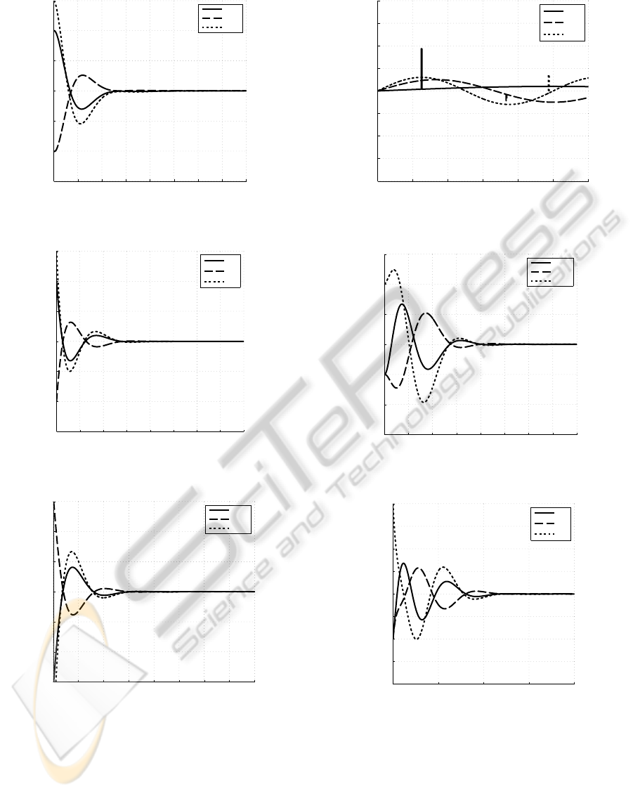
0 1 2 3 4 5 6 7 8

−3

−2

−1

Time [s]

Position tracking error [m]

l,1

l,2

l,3

Figure 2: Position tracking error of the leader spacecraft.

0 1 2 3 4 5 6 7 8

−3

−2

−1

Time [s]

Position estimation error [m]

˜p

Figure 3: Position estimation error of the leader spacecraft.

0 1 2 3 4 5 6 7 8

−600

−400

−200

200

400

600

Time [s]

Control history [N]

l,1

l,2

l,3

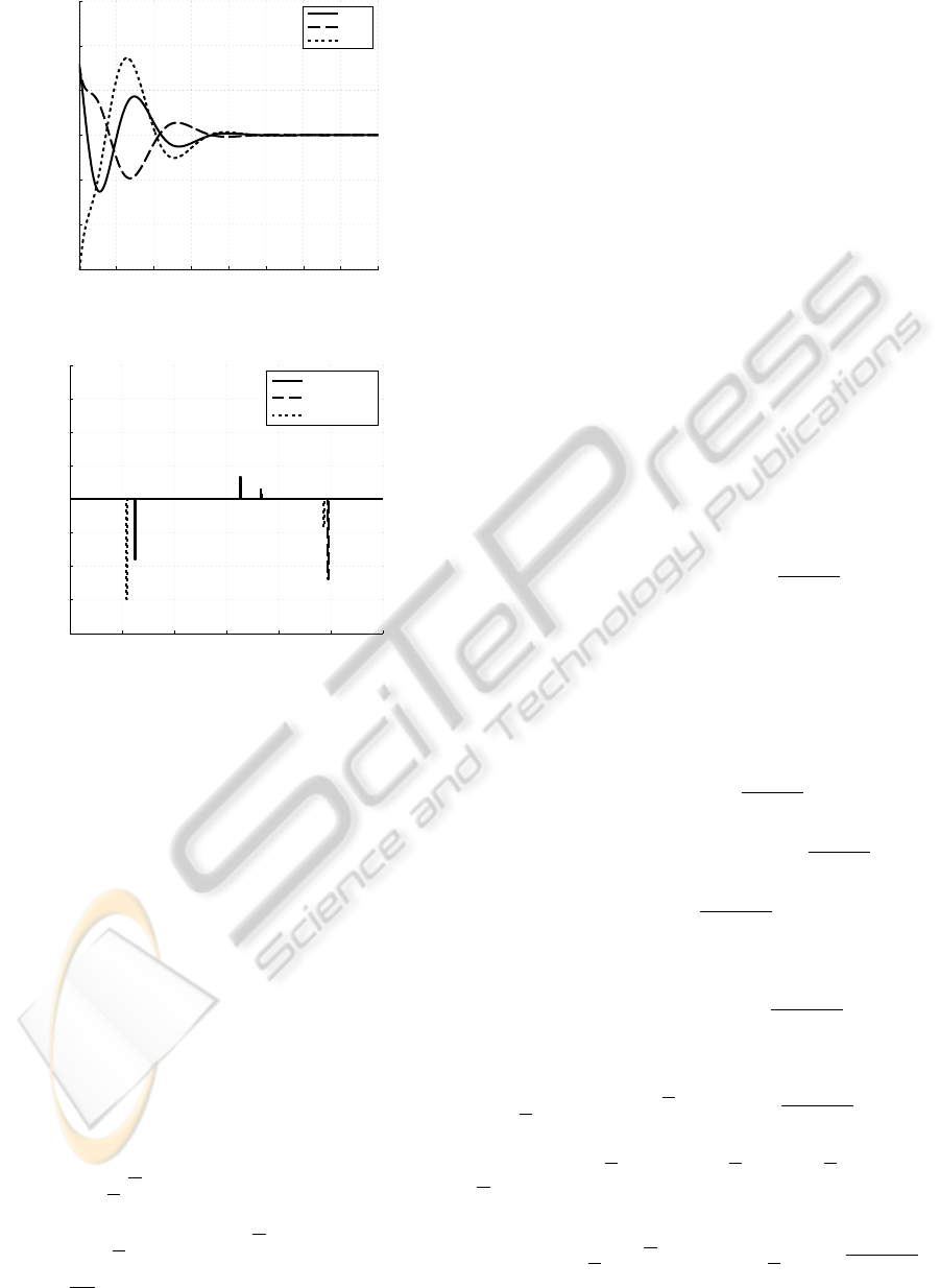
Figure 4: Control actuation of the leader spacecraft.

be shown that the disturbances satisfy the following:

t+10

|d(τ)|

dτ ≤ 1.42, ∀t ≥ 0 .

Figure 2, 3 and 4 show the position tracking er-

ror, position estimation error and control history of

the leader spacecraft, whereas Figure 6, 7 and 8 are

the equivalent ﬁgures for the follower spacecraft. Fig-

0 5 10 15 20 25 30

−2

−1.5

−1

−0.5

0.5

1.5

Time [s]

Disturbance [N]

l,1

l,2

l,3

Figure 5: Disturbances acting on the leader spacecraft.

0 1 2 3 4 5 6 7 8

−3

−2

−1

Time [s]

Position tracking error [m]

f,1

f,2

f,3

Figure 6: Position tracking error of the follower spacecraft.

0 2 4 6 8

−2

−1.5

−1

−0.5

0.5

1.5

Time [s]

Position estimation error [m]

˜ρ

Figure 7: Position estimation error of the follower space-

craft.

ure 5 and 9 show the effect of d

and d

−d

acting

on the formation. Notice in Figure 9 that the ef-

fect of the continuous part of the disturbance is can-

celed out (since we consider relative dynamics and

both spacecraft are inﬂuenced by the same continu-

ous disturbance), whereas the effect of the impacts

has increased compared to the effect of the impacts

ICINCO 2010 - 7th International Conference on Informatics in Control, Automation and Robotics

0 1 2 3 4 5 6 7 8

−600

−400

−200

200

400

600

Time [s]

Control history [N]

f,1

f,2

f,3

Figure 8: Control actuation of the leader spacecraft.

0 5 10 15 20 25 30

−2

−1.5

−1

−0.5

0.5

1.5

Time [s]

Disturbance [N]

l,1

− d

f,1

l,2

− d

f,2

l,3

− d

f,3

Figure 9: Disturbances acting on the follower spacecraft.

on the leader spacecraft. The control gains have been

chosen based on the Lyapunov analysis. This yields

in general very conservative constraints on the choice

of control gains, and also conservative estimates of

the disturbances the control system is able to handle.

As shown in Figure 4, and in particular Figure 8, this

leads to large transients in the actuation. We stress

that the control gains proposed by this approach is still

much smaller that those obtained through a classical

ISS approach (i.e. relying on the disturbance magni-

tude).

4 PROOF OF THEOREM 1

In view of (Praly and Wang, 1996, Lemma 11) and

(Angeli et al., 2000, Remark 2.4), there exists a con-

tinuously differentiable function V : R

→ R

≥0

, class

∞

functions α,α and γ, and a positive constant κ

such that, for all x ∈R

and all u ∈ R

α(|x|) ≤V (x) ≤ α(|x|) (30)

∂V

∂x

(x) f (x,u) ≤ −κV (x)+ γ(|u|) . (31)

Let w(t) := V (x(t; x

,u)). Then it holds in view of

(31) that

˙w(t) =

V (x(t;x

,u))

≤ −κV (x(t; x

,u)) + γ(|u(t)|)

≤ −κw(t) + γ(|u(t)|).

In particular, it holds that, for all t ≥ 0,

w(t) ≤ w(0)e

−κt

γ(|u(s)|)ds. (32)

Assuming that u belongs to the class W

(E, T ), for

some arbitrary constants E, T > 0, it follows that

w(T ) ≤w(0)e

−κT

γ(|u(s)|)ds ≤w(0)e

−κT

+E .

Considering this inequality recursively, it follows

that, for each ` ∈ N

≥1

w(`T ) ≤ w(0)e

−`κT

+ E

k−1

∑

j=0

−jκT

≤ w(0)e

−`κT

+ E

∑

j≥0

−jκT

≤ w(0)e

−`κT

+ E

κT

−1

. (33)

Given any t ≥ 0, pick ` as bt/T c and deﬁne t

:= t −

`T . Note that t

∈ [0,T ]. It follows from (32) that

w(t) ≤w(`T )e

−κt

γ(|u(s)|)ds ≤w(`T )e

−κt

+E ,

which, in view of (33), implies that

w(t) ≤



w(0)e

−`κT

+ E

κT

−1



−t

+ E

≤ w(0)e

−k(`T +t

)

+ E



1 +

κT

−1



≤ w(0)e

−κt

κT

−1

κT

−1

E .

Recalling that w(t) = V (x(t; x

,u)), it follows that

V (x(t;x

,u)) ≤V (x

−κt

κT

−1

κT

−1

E ,

which implies, in view of (30), that

α(|x(t;x

,u)|) ≤ α(|x

|)e

−κt

κT

−1

κT

−1

E ,

Recalling that α

−1

(a + b) ≤ α

−1

(2a) + α

−1

(2b) as

α ∈ K

∞

, we ﬁnally obtain that, given any x

∈ R

any u ∈ W

(E, T ) and any t ≥ 0,

|x(t;x

,u)|≤α

−1



2α(|x

|)e

−κt



+α

−1



κT

−1

κT

−1



(34)

ROBUSTNESS OF ISS SYSTEMS TO INPUTS WITH LIMITED MOVING AVERAGE, WITH APPLICATION TO

SPACECRAFT FORMATIONS

Given any T,δ ≥0, the following choice of E:

E(T, δ) ≤

(δ)

κT

−1

κT

−1

. (35)

ensures that

−1



κT

−1

κT

−1



≤ δ

and the conclusion follows in view of (34) with the

K L function

β(s,t) := α

−1



2α(s)e

−κt



, ∀s,t ≥ 0 .

REFERENCES

Angeli, D. and Ne

c, D. (2001). Power characterizations

of input-to-state stability and integral input-to-state

stability. IEEE Transactions on Automatic Control,

48:1298–1303.

Angeli, D., Sontag, E. D., and Wang, Y. (2000). A char-

acterization of integral input-to-state stability. IEEE

Transactions on Automatic Control, 45:1082–1097.

Berghuis, H. (1993). Model-based Robot Control: from

Theory to Practice. PhD thesis, Universiteit Twente.

Berghuis, H. and Nijmeijer, H. (1993). A passivity approach

to controller-observer design for robots. IEEE Trans-

actions on Robotics and Automation, 9(6):740–754.

Clohessy, W. H. and Wiltshire, R. S. (1960). Terminal

guidance system for satellite rendezvous. Journal of

Aerospace Sciences, 27:9.

une, L. (2002). Input-to-state dynamical stability and its

Lyapunov function characterization. IEEE Transac-

tions on Automatic Control, 47:1499–1504.

une, L. (2004). Quantitative aspects of the input-to-

state-stability property. In de Queiroz, M., Malisoff,

M., and Wolenski, P., editors, Optimal Control, Sta-

bilization and Nonsmooth Analysis, pages 215–230.

Springer-Verlag.

Hanslmeier, A., Denkmayr, K., and Weiss, P. (1999).

Longterm prediction of solar activity using the com-

bined method. Solar Physics, 184:213–218.

NASA (1999). On space debris. Technical report, NASA.

ISBN: 92-1-100813-1.

Overhage, C. F. J. and Radford, W. H. (1964). The Lin-

coln Laboratory West Ford Program - An historical

perspective. Proceeding of the IEEE, 52:452–454.

Paden, B. and Panja, R. (1988). Globally asymptotically

stable ’PD+’ controller for robot manipulators. Inter-

national Journal of Control, 47(6):1697–1712.

Ploen, S. R., Scharf, D. P., Hadaegh, F. Y., and Acikmese,

A. B. (2004). Dynamics of earth orbiting formations.

In Proc. of AIAA Guidance, Navigation and Control

Conference.

Praly, L. and Wang, Y. (1996). Stabilization in spite of

matched unmodeled dynamics and an equivalent deﬁ-

nition of input-to-state stability. Mathematics of Con-

trol, Signals, and Systems, 9:1–33.

Sch

afer, F. (2006). The threat of space debris and microm-

eteoroids to spacecraft operations. ERCIM NEWS,

(65):27–29.

Sontag, E. D. (1989). Smooth stabilization implies coprime

factorization. IEEE Transactions on Automatic Con-

trol, 34:435–443.

Sontag, E. D. (1998). Comments on integral variants of ISS.

Systems & Control Letters, 34:93–100.

Sontag, E. D. (2008). Input to state stability: Basic concepts

and results. In Nistri, P. and Stefani, G., editors, Non-

linear and Optimal Control Theory, pages 163–220.

Springer-Verlag, Berlin.

Sontag, E. D. and Wang, Y. (1995). On characterizations of

the input-to-state stability property. Systems & Con-

trol Letters, 24:351–359.

Wertz, J. R., editor (1978). Spacecraft attitude determi-

nation and control. D. Reidel Publishing company.

ISBN: 9027709599.

ICINCO 2010 - 7th International Conference on Informatics in Control, Automation and Robotics