ESTIMATING SOFTWARE DEVELOPMENT EFFORT USING

TABU SEARCH

Filomena Ferrucci, Carmine Gravino, Rocco Oliveto and Federica Sarro

Dipartimento di Matematica e Informatica, Università di Salerno, Via Ponte Don Melillo, Fisciano (SA), Italy

Keywords: Development Effort Estimation, Empirical Studies, Tabu Search.

Abstract: Some studies have been recently carried out to investigate the use of search-based techniques in estimating

software development effort and the results reported seem to be promising. Tabu Search is a meta-heuristic

approach successfully used to address several optimization problems. In this paper, we report on an

empirical analysis carried out exploiting Tabu Search on two publicly available datasets, i.e., Desharnais

and NASA. On these datasets, the exploited Tabu Search settings provided estimates comparable with those

achieved with some widely used estimation techniques, thus suggesting for further investigations on this

topic.

1 INTRODUCTION

Effort estimation is a critical basic activity for

planning and monitoring software project

development and for delivering the product on time

and within budget. Several methods have been

proposed in order to estimate software development

effort. Many of them determine the prediction

exploiting some relevant factors of the software

project, named cost drivers. These methods, named

data-driven, exploit data from past projects,

consisting of both factor values that are related to

effort and the actual effort to develop the projects, in

order to estimate the effort for a new project under

development (Shepperd and Schofield, 2000). In this

class, we can find some widely used techniques,

such as Linear and Stepwise Regression,

Classification and Regression Tree, and Case-Based

Reasoning (Briand and Wieczorek, 2002).

In the last years, some attempts have been made

to apply search-based approaches to estimate

software development effort. Indeed, effort

estimation can be formulated as an optimization

problem (Harman, 2007), where we have to search

for the most accurate estimate, i.e. the one that

minimizes the difference with the actual effort. In

particular, some researchers have analyzed the use

of Genetic Programming in estimating software

development effort (Burgess and Lefley, 2001)

(Lefley and Shepperd, 2003), reporting results that

encourage further investigations in this context.

Genetic Programming is a search-based approach

inspired by evolutionary biology to address

optimization problems. There exist other search-

based techniques that have been found to be very

effective and robust in solving numerous

optimization problems. In particular, Tabu Search

has been successfully applied for software testing

(Diaz et al., 2008), for object replication in

distributed web server (Mahmood and Homeed,

2005) and for Software-Hardware Partitioning

(Lanying and Shi, 2008). In this paper, we report on

an empirical study carried out to analyze the

effectiveness of Tabu Search for effort estimation. In

particular, the specific contributions of the paper are:

 the definition and the analysis of a Tabu Search

algorithm for effort estimation;

 the comparison of the proposed approach with

widely used estimation methods.

To this aim we employed two publicly available

datasets, i.e., Desharnais (Desharnais, 1989) and

NASA (Bailey and Basili, 1981), widely used in the

context of effort estimation.

The remainder of the paper is organized as

follows. Section 2 provides a brief description of the

Tabu Search algorithm conceived for estimating

software development effort. Section 3 summarizes

the empirical analysis we performed to assess the

effectiveness of the algorithm. Related work is

presented in Section 4. Final remarks and future

work conclude the paper.

236

Ferrucci F., Gravino C., Oliveto R. and Sarro F. (2010).

ESTIMATING SOFTWARE DEVELOPMENT EFFORT USING TABU SEARCH.

In Proceedings of the 12th International Conference on Enterprise Information Systems - Databases and Information Systems Integration, pages

236-241

DOI: 10.5220/0002901002360241

 SciTePress

2 THE ESTIMATION METHOD

Tabu Search (TS) is an optimization method

proposed originally by Glover to overcome some

limitations of Local Search (Glover and Laguna,

1997). It is a meta-heuristic relying on adaptive

memory and responsive exploration of the search

space. To build a TS algorithm we have to perform

the following steps:

 define a representation of possible solutions;

 define the neighbourhood;

 choose an objective function to evaluate

solutions;

 define the Tabu list, the aspiration criteria, and

the termination criteria.

In the context of effort estimation, a solution

consists of a model described by an equation that

combines several factors:

Effort = c

... op

2n−2

2n−1

where f

and c

represent the values of the i

factor

and its coefficient, respectively, C represents a

constant, while op

represents the i

operator.

Although a variety of operators could be considered,

only the set { + , - , * } was took into account for our

analysis.

The search space of TS is represented by all the

possible equations that can be generated assigning

the values for c

, C, op

providing positive Effort

values. The initial solution is randomly generated.

Starting from the current solution, at each iteration

the method applies local transformations (i.e.,

moves), defining a set of neighboring solutions in

the search space. Each neighbour of a given solution

S is defined as a solution obtained by a random

variation of it. In particular, a move consists of three

steps:

1. change each coefficient c

of S with probability

½. The new coefficient is calculated as follow:

),( r

c 



where



/,*,,f

and r is randomly chosen

in the range ]0,1];

2. change the constant factor C of S with

probability ½ in the same way coefficients are

changed;

3. change each arithmetic operator op

of S with

probability ½.

At each iteration the neighbouring solutions are

compared to select the best one which will be used

in the next iteration to explore a new neighbourhood.

Moreover, if the best neighbouring solution is better

than the current best solution, the latter is replaced.

The comparison between solutions is performed by

exploiting an objective function able to evaluate the

accuracy of the estimation model. A number of

accuracy measures are usually taken into account to

compare effort estimation models. All are based on

the residual, i.e. the difference between the predicted

and actual effort. Among them we used as objective

function the MMRE (Conte et al., 1986), whose

definition is reported in the next section. In

particular, the goal of TS is to minimize the MMRE

value.

To avoid loops and to guide the search far from

already visited portions of the search space; the

moves recently applied are marked as tabu and

stored in a Tabu list. Since only a fixed and fairly

limited quantity of information is usually recorded in

the Tabu list (Gendreau, 2002), we prohibit the use

of a tabu move for ten iterations. In order to allow

one to revoke a tabu move, we employed the most

commonly used aspiration criterion, namely we

permit a tabu move if it results in a solution with an

objective function value (i.e., the MMRE value)

better than the one of the current best solution.

The search is stopped after a fixed number of

iterations or after some number of iterations that do

not provide an improvement in the objective

function value.

3 EMPIRICAL ANALISYS

The goals of our empirical analysis were:

1) analyzing the effectiveness of TS in estimating

software development effort;

2) comparing the accuracy of TS with the one of

widely and successfully employed estimation

methods.

To evaluate the accuracy of the estimates we

employed some widely used summary measures

(Conte et al., 1986), namely: the Mean and Median

of Magnitude of Relative Error (MMRE and

MdMRE), and Pred(25). According to (Conte,

1986), a good effort prediction model should have a

MMRE≤0.25 and Pred(25)≥0.75, meaning that at

least 75% of the predicted values should fall within

25% of their actual values.

To address the second research goal, we

compared TS with Manual Stepwise Regression

(MSWR) (Kitchenham and Mendes, 2004) and

Case-Based Reasoning (CBR) (Shepperd and

Schofield, 2000), that are widely used estimation

techniques.

ESTIMATING SOFTWARE DEVELOPMENT EFFORT USING TABU SEARCH

237

SWR is a statistical technique that allows us to

build a prediction model representing the

relationship between independent and dependent

variables. The estimation model is obtained by

adding, at each stage, the independent variable with

the highest association to the dependent variable,

taking into account all variables currently in the

model. SWR aims to find the set of independent

variables that best explains the variation in the

dependent variable.

To select the variables to be added in the model a

Manual SWR (MSWR) can be applied, using the

technique proposed by Kitchenham (1998). The idea

underlying this procedure is to select the important

independent variables, and then to use linear

regression to obtain the final model.

CBR is a branch of Artificial Intelligence where

knowledge of similar past cases is used to solve new

cases. The idea is to predict the effort of a new

project by considering similar projects previously

developed. We applied CBR by employing ANGEL

(Shepperd and Schofield, 2000). ANGEL

implements the Euclidean distance as similarity

function and uses features normalised between 0 and

1. We used 1, 2, and 3 analogies employing as

adaptation strategies the mean of k analogies (simple

average), the inverse distance weighted mean and

the inverse rank weighted mean (Shepperd and

Schofield, 2000). We used the feature subset

selection of ANGEL in order to let the tool to

automatically choose, among all the variables, the

ones to employ as set of key features in the analogy

based estimation.

To have a better visual insight on the

effectiveness of the estimation models, we compared

the prediction accuracies taking into account both

the summary statistics and the boxplots of absolute

residuals, where residuals are calculated as (EFreal –

EFpred). Boxplots are widely employed in

exploratory data analysis since they provide a quick

visual representation to summarize the data, using

five values: median, upper and lower quartiles,

minimum and maximum values, and outliers

(Kitchenham et al., 2001). In development effort

estimation, boxplots are used to visually represent

the amount of the error for a given prediction

technique. In particular, we used boxplot to

graphically render the spread of the absolute

residuals.

In order to verify whether the estimates obtained

with TS are characterized by significantly better

accuracy than the considered benchmarks we

statistically analyzed the absolute residuals, as

suggested in (Kitchenham et al., 2001). Since (i) the

absolute residuals for all the analyzed estimation

methods were not normally distributed, and (ii) the

data was naturally paired, we decided to use the

Wilcoxon test (Royston, 1982). The achieved results

were intended as statistically significant at = 0.05.

We performed the empirical analysis by

exploiting two datasets: the Desharnais (Desharnais,

1989) dataset, containing 81 observations, and the

NASA (Bailey and Basili, 1981) dataset, with 18

observations. Despite of these datasets are quite old,

they have been widely and recently used to evaluate

and compare estimation methods (see e.g., (Burgess

and Lefley, 2001) (Shepperd and Schofield, 2000)).

As for Desharnais dataset, in our analysis we did not

consider the length of the code as made in (Burgess

and Lefley, 2001), and categorical variables (i.e.,

Language and YearEnd). We excluded four projects

that had missing values, as done by Shepperd and

Schofield (2000). The NASA dataset consists of two

independent variables, i.e. Developed Lines (DL) of

code and Methodology (Me). The descriptive

statistics of the selected factors for the two datasets

are shown in Tables 1 and 2.

Table 1: Descriptive statistics of Desharnais dataset.

Variable Min Max Mean Std.Dev.

TeamExp 0.00 4.00 2.30 1.33

ManagerExp 0.00 7.00 2.65 1.52

Entities 7.00 387.00 120.55 86.11

Transactions 9.00 886.00 177.47 146.08

AdjustedFPs 73.00 1127.00 298.01 182.26

RawFPs 62.00 1116.00 282.39 186.36

Envergue 5.00 52.00 27.45 10.53

EFH (m/h) 546.00 23490.00 4903.95 4188.19

Table 2: Descriptive statistics of NASA dataset.

Variable Min Max Mean Std. Dev.

Me 19.00 35.00 27.78 5.39

DL 2.10 100.80 35.26 35.10

EFH (m/m) 5.00 138.30 49.47 45.73

We exploited some parameter settings to find

suitable values for moves and iterations numbers.

Concerning the number of moves, we executed TS

using four different values, i.e. 100, 500, 1000, and

2000. The best results in terms of MMRE and

Pred(25) were achieved with 1000 moves for

Desharnais dataset and 100 moves for NASA

dataset. We also executed the algorithm with

different numbers of iterations, and the best results

were achieved using 3000 and 500 iterations on

Desharnais and NASA, respectively. We did not

consider number of moves greater than 2000 for

Desharnais dataset and 100 for NASA dataset since

we noted a decreasing in the performance.

Moreover, note that for NASA dataset, having a

ICEIS 2010 - 12th International Conference on Enterprise Information Systems

238

number of factors and observations less than the

Desharnais dataset, the best results were obtained

with fewer moves. This aspect should be further

investigated in the future using other datasets to

verify whether some thresholds could be identified

in the choice of moves number. A similar

consideration can be made for the number of

iterations.

The validation process was performed using a

hold-out validation on Desharnais and a 3-fold cross

validation for NASA, since it is quite small (Briand

and Wieczorek, 2002). In particular, we randomly

split the Desharnais dataset into a training set of 59

observations and a test set of 18 observations.

NASA dataset was partitioned into 3 randomly test

sets of equal size and then for each test set we used

the remaining 12 observations as training set.

Table 3 and Table 4 provide the results for the

summary measures MMRE, MdMRE, and Pred(25).

As we can see the thresholds provided in (Conte,

1986) are not satisfied for TS on Desharnais, since

Pred(25) value is less than 0.75 and MMRE and

MdMRE values are greater than 0.25. On the other

hand, the estimates obtained on NASA provided

MMRE and MdMRE values less than 0.25 and a

Pred(25) value very close to 0.75.

To have an insight on the results and understand

the actual effectiveness of TS on these datasets, it is

important to compare TS estimation accuracy with

that of widely used techniques, such as MSWR and

CBR (reported in Tables 3 and 4). Only the best

results obtained for CBR are reported.

Table 3: MMRE, MdMRE, and Pred(25) on Desharnais.

MMRE PRED(25) MdMRE

TS 0.45 0.39 0.43

CBR 0.48 0.55 0.22

MSWR 0.39 0.22 0.38

Table 4: MMRE, MdMRE, and Pred(25) on NASA.

MMRE PRED(25) MdMRE

TS 0.21 0.72 0.19

CBR 0.24 0.56 0.20

MSWR 0.20 0.72 0.19

Table 5: Results of Wilcoxon tests.

TS vs MSWR TS vs CBR

Desharnais p-value = 0.41 p-value = 0.16

NASA p-value= 0.80 p-value = 0.17

As for Desharnais, we can see that TS provided a

better Pred(25) value and slightly worse MMRE and

MdMRE values with respect to MSWR. As for

CBR, TS achieved a slightly better MMRE value but

worse MdMRE and Pred(25) values. Regarding the

NASA dataset, the best results were achieved using

MSWR and TS, while the worse results were

obtained with CBR. In particular, TS and MSWR

provided comparable results.

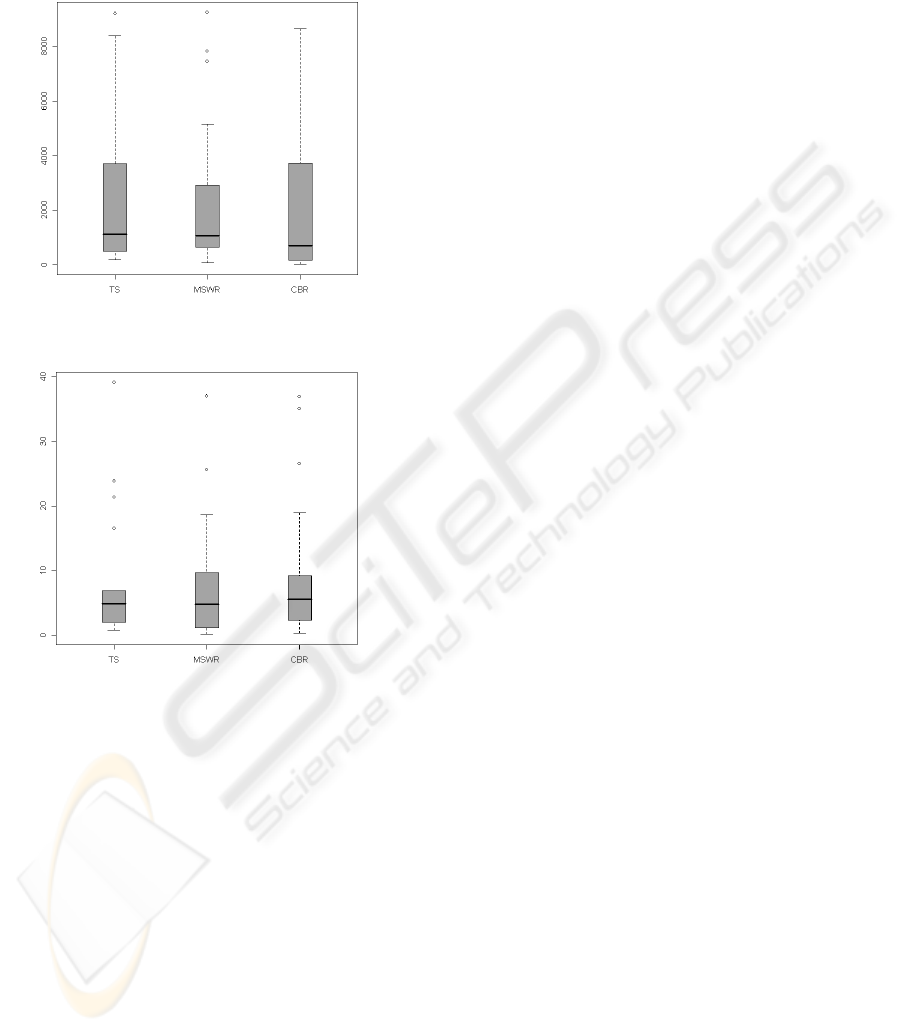
The analysis of the boxplots in Figures 1 and 2

suggests that TS has a median very close to the

median of MSWR and CBR. With regards to

Desharnais dataset, even if the boxplot of MSWR is

less skewed than those of CBR and TS, it has more

outliers. Furthermore, the boxes and the tails of TS

and CBR are quite similar. As for NASA dataset, the

tails of TS boxplot are less skewed and the outliers

of TS are more close to the box. In the other cases,

the box length and tails of boxplots are similar.

Summarizing, we can deduce that boxplot of TS is

slightly better than the boxplots of CBR and MSWR

for NASA dataset.

To get a better understanding, we also tested the

statistical significance of the results by comparing

paired absolute residuals with the Wilcoxon test (see

Table 5). We can observe that for both datasets,

there is no statistical significant difference between

the absolute residuals obtained with TS and CBR

and TS and MSWR (the results were intended as

statistically significant at α = 0.05). Thus, we can

conclude that for the performed analysis TS has

comparable performances with respect to two widely

used estimation techniques.

However, further analysis could be carried out to

identify a better setting of the features of the TS

algorithm. Indeed, for example other operators could

be used for the prediction model, as well as other

measures could be exploited as objective function

instead or together with MMRE.

It is interesting to compare our results with the

one of Burgess and Lefley (2001) that assessed the

use of Genetic Programming (GP) for estimating

software development effort exploiting on the

Desharnais dataset. The settings they used were: an

initial population of 1000, 500 generations, 10

executions (i.e., run), and a fitness function designed

to minimize MMRE. The proposed GP did not

outperform Linear Regression (LR), CBR (with k=2

and k=5 analogies), and Artificial Neural Networks

(ANN) in terms of summary measures MMRE and

Pred(25). However, no statistical tests were carried

out by the authors to verify whether there was

significant difference between the results. As for GP,

they obtained an MMRE value which is close to the

one we obtained with TS, and a Pred(25) value

which is worse than the one obtained with TS.

So, our analysis confirms their results on the

potentially effectiveness of search-based techniques

for effort estimation by suggesting also the

ESTIMATING SOFTWARE DEVELOPMENT EFFORT USING TABU SEARCH

239

usefulness of TS. Moreover, it confirms the need for

further investigations to verify if a better set up of

the algorithms could improve the accuracy of the

estimations.

Figure 1: The boxplots of absolute residuals, Desharnais

dataset.

Figure 2: The boxplots of absolute residuals, NASA

dataset.

4 RELATED WORK

Besides, the work of Burgess and Lefley (2001)

whose results have been reported in Section 3, some

empirical investigations have been performed to

assess the effectiveness of genetic algorithms in

estimating software development effort. In

particular, Dolado (2000) employed an evolutionary

approach in order to automatically derive equations

alternative to multiple linear regression. The aim

was to compare the linear equations with those

obtained automatically. The proposed algorithm was

run a minimum of 15 times and each run had an

initial population of 25 equations. Even if in each

run the number of generation varied, the best results

were obtained with three to five generations (as

reported in the literature, usually more generations

are used) and by using the Mean Squared Error

(MSE) (Conte et al., 1986), as fitness function. As

dataset, 46 projects developed by academic students

were exploited through a hold-out validation. It is

worth noting that the main goal of Dolado work was

not the assessment of evolutionary algorithms but

the validation of the component-based method for

software sizing. However, he observed that the

investigated algorithm provided similar or better

values than regression equations.

Successively, Lefley and Shepperd (2003) also

assessed the effectiveness of an evolutionary

approach and compared it with several estimation

techniques such as LR, ANN, and CBR. As for

genetic algorithm setting, they applied the same

choice of Burgess and Lefley (2001), while a

different dataset was exploited. This dataset is

refereed as “Finnish Dataset” and included 407

observations and 90 features, obtained from many

organizations. After a data analysis, a training set of

149 observations and a test set of 15 observations

were obtained applying a hold-out validation and

used in the empirical analysis. Even if the results

revealed that there was not a method that provides

better estimations than the others, the evolutionary

approach performed consistently well.

An evolutionary computation method, named

Grammar Guided Genetic Programming (GGGP),

was proposed by Shan et al. (2002) to fit models,

with the aim of improving the estimation of the

software development effort. Data of software

projects from ISBSG database was used to build the

estimation models using GGGP and LR. The fitness

function was designed to minimize the Mean

Squared Error (MSE), an initial population of 1000

was chosen, the maximum number of generations

was 200, and the number of executions was 5. The

results revealed that GPPP performed better than

Linear Regression in terms of MMRE and Pred(25).

5 CONCLUSIONS AND FUTURE

WORKS

Our analysis has shown that Tabu Search can be

effective as other widely used estimation techniques.

The study can be seen as a starting point for further

investigations to be carried out (possibly with other

datasets) by taking into account several different

configuration settings of TS. These configurations

could be based on:

 several objective functions possibly not em-

ICEIS 2010 - 12th International Conference on Enterprise Information Systems

240

ployed in the previous works. Indeed, such a

choice could influence the achieved results

(Harman, 2007), particularly when the measure

used by the algorithm to optimise the estimates is

the same used to evaluate the accuracy of them

(Burgess and Lefley, 2001). Moreover, we could

consider a multi-objective optimisation given by

a combination of Pred(25) and MMRE.

 other operators and moves to better explore the

solution space.

We will also replicate the study employing data

from other companies in order to mitigate possible

external validity threats (Briand and Wust, 2001).

ACKNOWLEDGEMENTS

The research has also been carried out exploiting the

computer systems funded by University of Salerno’s

Finanziamento Medie e Grandi Attrezzature (2005)

for the Web Technologies Research Laboratory.

REFERENCES

J. W. Bailey, V. R. Basili, 1981. A Meta Model for

Software Development Resource Expenditure. Procs.

of Conference on Software Engineering, pp. 107-115.

L. Briand, I. Wieczorek, 2002. Software Resource

Estimation. Encyclopedia of Software Engineering.

Volume 2. P-Z (2nd ed.), Marciniak, John J. (ed.) New

York: John Wiley & Sons, pp. 1160-1196.

L. C. Briand, J. Wust, 2001. Modeling Development

Effort in Object-Oriented Systems Using Design

Properties. IEEE TSE, 27(11), pp. 963–986.

L. Briand, K. El. Emam, D. Surmann, I. Wiekzorek, K.

Maxwell, 1999. An assessment and comparison of

common software cost estimation modeling

techniques. Procs. Conf. on Software Engineering, pp.

313–322.

C. Burgess, M. Lefley, 2001. Can Genetic Programming

Improve Software Effort Estimation: a Comparative

Evaluation. Inform. Softw. Technology, 43(14), pp.

863–873.

D. Conte, H. Dunsmore, V. Shen, 1986. Software

engineering metrics and models. The

Benjamin/Cummings Publishing Company, Inc..

J. M. Desharnais, 1989. Analyse statistique de la

productivitie des projets informatique a partie de la

technique des point des function. Unpublished Masters

Thesis, University of Montreal.

E. Diaz, J. Tuya, R. Bianco, J. J. Dolado, 2008. A tabu

search algorithm for structural software testing. Comp.

and Oper. Research, 35(10), pp. 3052-3072.

J. J. Dolado, 2000. A validation of the component-based

method for software size estimation. Transactions on

Software Engineering, 26(10), pp. 1006–1021.

M. Gendreau, 2002. An introduction to Tabu Search.

Inter’l Series in Operations Research & Management,

Science Handbook of Metaheuristics, 57, Springer, pp.

37-54.

F. Glover, M. Laguna, 1997. Tabu Search. Kluwer

Academic Publishers, Boston.

M. Harman, 2007. The Current State and Future of Search

Based Software Engineering. Workshop on the Future

of Software Engineering (ICSE’07), pp. 342-357.

B. A. Kitchenham, 1998. A procedure for analyzing

unbalanced datasets. Transactions on Software

Engineering, 24 (4), pp. 278-301.

B. Kitchenham, L. M. Pickard, S. G. MacDonell, M. J.

Shepperd, 2001. What accuracy statistics really

measure. IEEE Procs. Software 148(3), pp. 81–85.

L. Lanying, M. Shi, 2008. Software-Hardware Partitioning

Strategy Using Hybrid Genetic and Tabu Search.

Procs. Conf. Computer Science and Software

Engineering, Vol. 04, pp. 83-86.

M. Lefley, M. J. Shepperd, 2003. Using genetic

programming to improve software effort estimation

based on general data sets. Procs. of Genetic and

Evolutionary Computation Conf., pp. 2477–2487.

A. Mahmood, T. Homeed, 2005. A Tabu Search

Algorithm for Object Replication in Distributed Web

Server System. Studies in Informatics and Control,

14(2), pp. 85-98.

P. Royston, 1982. An extension of Shapiro and Wilks Test

for Normality to Large Samples. Applied Statistics

31(2), pp. 115–124.

Y. Shan, R. I. Mckay, C. J. Lokan, D. L. Essam, 2002.

Software project effort estimation using genetic

programming. Procs. of Conf. on Communications

Circuits and Systems, pp. 1108–1112.

M. Shepperd, C. Schofield, 2000. Estimating software

project effort using analogies. IEEE TSE, 23(11), pp.

736–743.

L. J. White, 2002. Editorial: The importance of empirical

work for software engineering papers. Software

Testing, Verification and Reliability, 12 (4), pp. 195-

196.

ESTIMATING SOFTWARE DEVELOPMENT EFFORT USING TABU SEARCH

241