
MOTION GENERATION FOR A HUMANOID ROBOT WITH
INLINE-SKATE
Nir Ziv*, Yong Kwun Lee* and Gaetano Ciaravella**
*Center for Cogntive Robotics, University of Science and Technology (UST) & Korea Institute of Science and Technology
(KIST), 39-1 Hawolgol-Dong, Wolsong-Gil 5, Seongbuk-gu, Seoul, South Korea
**Cognative Center for Robotic Research, Korea Institute of Science and Technology (KIST), Seoul, South Korea
Keywords: Humanoid, Inline-Skate, Skating Motion, Wheeled Locomotion.
Abstract: A lot of research has been done for bipedal walking and many positive results have been produced, such as
the ASIMO robot from Honda. However, although bipedal walking is a good solution for moving over
uneven surfaces; bipedal walking is inefficient over an even surface because the robot’s walking speed and
stability are limited. Consequently, employing a wheeled locomotion on even surfaces can be advantageous.
This paper presents a mathematical model and simulation of wheeled biped robot with two passive wheels
on each foot. This enables the robot to move more efficiently over even surfaces. Also, this paper attempts
to produce a more human-like inline-skating motion than previously created inline-skating simulations.
1 INTRODUCTION
Over the last few years, research on bipedal walking
has progressed and has lead to major successes
within the robotics field. One good example of this
success is the ASIMO robot, a Honda creation. At
the time of writing this paper, ASIMO can run with
a speed of 6 km/h and is able to walk at a speed of
2.7 km/h (Honda). When considering the strongest
achievements which leg locomotion has achieved
until now, one major progressive accomplishment
has been the ability for robots to move across
uneven surfaces.
However, when considering robotic leg
locomotion across only even tarains, the advantages
of wheeled locomotion are greater than bipedal (or
leg) locomotion. The reason for this is because the
wheeled robot’s moving speed and efficiancy are
stronger and more stable. This is because leg
locomotion algorithms are more complex than
wheeled motion, making it more difficult for bipedal
robots to walk or run quickly. (Jo et al 2008).
Therefore, to combine the advantages of both leg
and wheeled locomotion, hybrid robot systems were
developed. For example, WorkPartner is a
quadruped system that can detect the type of surface
it is on, even or uneven, and can then choose
accordingly the type of locomotion to use, wheeled
or bipedal (Ylonen et al 2002). Another example of
hybrid locomotion is WS-2/ WL-16 (Waseda Shoes
– Number 2 / Waseda Leg – Number 16)
(Hashimoto et al 2005) which also combines bipedal
walking with wheeled locomotion. Both
WorkPartner and WS-2/WL-16 use DC motorized
wheels.
However, because both WorkPartner and WS-
2/WL-16 utilize motor wheels, this means that the
brake and steering are also motorized. As a result, a
robot with motorized wheels has larger wheels and
its robotic system becomes heavier and, therefore,
less agile.
To solve this issue, passive wheel locomotion
has been suggested. One example of a hybrid,
passive wheeled robot is the Roller-walker,
developed by Hirose and Takeuchi (Hirose et al
1996, 1999, 2000.) In this system, the wheel motion
is not generated by a DC motor, instead the robot
moves by making a roller skating-like motion.
Another example of passive wheel locomotion is the
Rollerblader (Chitta et al 2003), which has two
passive wheels that move in symmetric and anti-
symmetric motions to propel the Rollerblader
forward and in a rotary motion respectively.
Similarly, in this paper we present a simulation
of a passive wheeled robot to generate a forward
motion; our robot consists of two legs with two
passive wheels attached along the middle of each
354
Ziv N., Lee Y. and Ciaravella G. (2010).
MOTION GENERATION FOR A HUMANOID ROBOT WITH INLINE-SKATE.
In Proceedings of the 7th International Conference on Informatics in Control, Automation and Robotics, pages 354-359
Copyright
c
SciTePress
foot. However, unlike the Rollerblader, our
simulation and model will attempt to create a more
human-like motion using ‘D’ shape movement for
the pushing leg where near the end of the movement
the pushing leg will be raised in the air.
This paper is organized as follows. The
following section will describe the modelling and
the equations of the robot’s motion. In section 3, we
will show the simulation, motion steps and results.
We will conclude with a brief discussion about the
simulation’s results, as well as problems that need to
be solved within further research in the future.
2 MODELLING
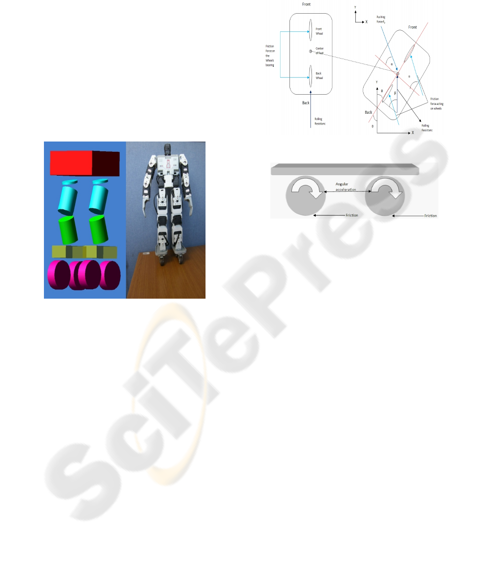
Figure 1: MSC.ADAMS Model and Read Small Size
Humanoid.
The modelling of the robot (figure 1) was done by
using MSC.ADAMS software. The robot has a total
of 12 Degrees Of Freedom (DOF), where each leg
contains 6 DOF. Two passive wheels were added to
each foot along the middle of the foot.
The forces acting on the robot configuration
(figure 2) and a derivation of the equations of
motion are shown and explained in more detail in
the next section.
2.1 Parametric Modelling
Solving the equations of motion for this system is a
very complex process; therefore, the following few
assumptions were made:
Even though the motion is continuous, we will
solve it for a time equal to t (where t is a segment of
the whole motion.)
External force, such as air resistance, external
push and wind are negligible.
The simulation motion is a forward motion.
This will reduce the amount of forces acting on the
model for rotational motion.
Figure 2: Forces Acting on the Robot.
Figure 3: Side View of the Forces Acting on the Robot.
Because we are trying to simulate a forward
motion, the forces acting on the model should satisfy
the following equations:
0
(1)
F
M
y
(2)
Where F
x
and F
y
are the forces acting on the X
axis and Y axis respectively. M
t
is the total mass and
y is acceleration. As figure 2 shows, we will
calculate the forces that act on the model.
First, we will analyze the stationary foot. Figure
2 shows the robot’s stationary foot as the left foot.
(3)
NM
g
Where F
r
, C
rr
and N are the rolling resistance
force, the rolling resistance coefficient and the
normal force respectively (Peck et al 1859,National
Research council 2006) and, in this instance, the
normal force is total mass (M
t
) times gravity (g).
(4)
Where F
fs
is the frictional force on the stationary
MOTION GENERATION FOR A HUMANOID ROBOT WITH INLINE-SKATE
355

foot, µ
f
is the friction coefficient, N is the normal
force, M
t
is the total mass and g is the gravitational
force.
Because the stationary foot will always point
forward (there is no Z axis rotation) and the foot will
be perpendicular to the ground, the rolling resistance
force will always act on the Y axis. The frictional
force from equation (4) will be used for the wheels’
momentum as described next.
The last force acting on the stationary foot is the
wheels momentum force. This can be seen in figure
3. The force acting on the wheels can be expressed
as follows:
(5)
MO
w
is single wheel momentum, I is the inertial
mass,
is angular acceleration F
fs
is frictional force
on the stationary foot and r is the wheel radius.
Because we have two wheels on each foot, we can
express equation (5) as follows:
(6)
MO
t
is the total momentum force acting on the
stationary foot’s wheels.
Until now we have described the forces which
are acting on the stationary foot (or the left foot from
figure 2). Now we will describe in the same manner
the forces acting on the pushing foot (or the right
foot from figure 2).
First, we will look at the pushing force. The
pushing force will act on the pushing leg with an
angle of α. This angle will vary with time. However,
as stated earlier to simplify the equations, we assume
that we are looking at a given time t and therefore
remove the dependency of time.
Because the pushing force is acting with an
angle, we will need to derive the X and Y
component of this force. These components are as
follows:
(7)
F
px
and F
py
are the pushing forces on the X axis
and the Y axis respectively. F
p
is the pushing force
and α is the angle between the pushing force and the
pushing foot.
As a reaction force to the pushing force, the
pushing foot will experience a frictional force as
well. This force can be written as:
(8)
As with the pushing force, we will need to work
on the X axis and Y axis components of the friction
force. Using equation 8 with angle α produces the
following equations:
(9)
Where F
fpx
is the frictional force on the pushing
foot on the X axis and F
fpy
is on the Y axis.
Using equations (1) and (2) and summing all the
forces that act on the X axis and Y axis, we can
rewrite equations (1) and (2) as follows:
(10)
(11)
Using equations (3) – (9) and solving equation
(11) for , we can rewrite equation (11) as follows:
(12)
(13)
(14)
(15)
(16)
Where
,
and
.
For a full derivation of how we developed equation
(12), please refer to the appendix.
2.2 Model Analysis
From equation (16) above, we notice that in order to
make the acceleration higher, and therefore make the
robot move forward faster, we needed to identify a
few components of the equation and check the
values that qualify our needs.
Equation (16) can be written in simple form as
follows:
(17)
ICINCO 2010 - 7th International Conference on Informatics in Control, Automation and Robotics
356
Where:
(18)
(19)
2
sinC
cos sin
(20)
In order to make ÿ bigger, we must make A and
B bigger and make C as small as possible. To make
equation (18) bigger, we identified α as the variable
since F
p,
M
t
and µ are constants. Using this notion,
we plotted equation (18) into Matlab. The results are
shown in figure 4.
As can be seen in figure 4, which shows when α
is static and not dynamically changed by time, the
value of α that will be the best in order to make the
pushing force greatest ( i.e. part A) is α =
or ,in
other words, when α = 90
o
. At the same time, the
best value for µ is 0.2. When looking in detail at
equation (20), we identified α and β as the variables
because the rest of equation (20) is constant.
Because we already determined the value of α from
equation (18), we will need to find the best value of
β. Using the same value of α with β, we will succeed
to minimize equation (20) since cos (90
o
) will make
the last part of C equal to zero.
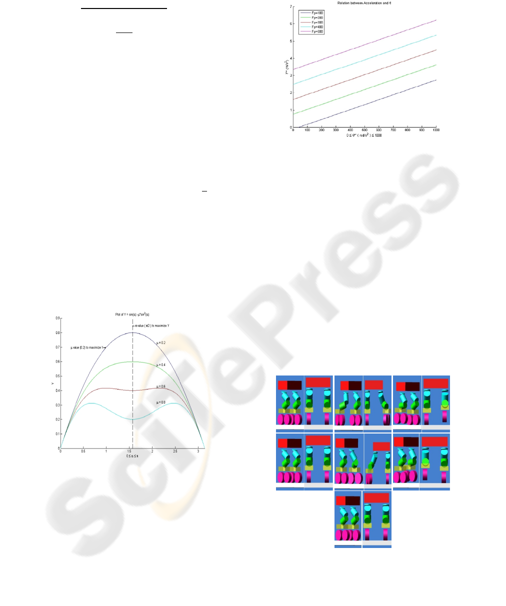
Figure 4: Matlab Plotting the relationship between values
of µ and α to maximize pushing force.
The middle part of equation (18) is shown in
equation (19) and has been plotted in Matlab; it can
be seen in figure 5. In figure 5, we showed the
relationship between the angular acceleration,
, and
the robot acceleration, ÿ. As expected, the
relationship between the two accelerations is linear,
which means that the faster the angular acceleration
on the wheels will be, the faster the robot
acceleration will be. Also, we verified the equations
with different values of the pushing force.
Figure 5: Matlab plotting the relationship between
acceleration and angular acceleration.
3 SIMULATION
We used MSC.ADAMS to simulate the skating
motion. The model is a simple model of the real
humanoid (see figure 1) and the motions were
generated by using three general motions that act on
the model (one general motion on the hip with
relation to the ground, one general motion on the left
leg with relation to the hip and the last general
motion on the right leg with relation to the hip as
well). With these three general motions we
controlled the angles or the joint and displacements
of the rigid bodies. The skating motion is combined
of six steps, three for the right foot, and three for the
left foot to produce a full cycle of motion.
Figure 6: The Simulation Algorithm Sequence. The left
image in each square shows the view from the side and the
image on the right shows the view from the back.
The shape of the pushing leg motion is like a ‘D’
MOTION GENERATION FOR A HUMANOID ROBOT WITH INLINE-SKATE
357
shape, starting from the top left corner and can be
viewed in two parts. In the first part, the pushing leg
is on the ground and is moving in slow motion. In
the second part, the pushing leg is in the air and to
maintain balance this step part is faster than the first
part of the cycle.
The following are the motion steps (assuming
that we begin with the right foot):
1. To start, the right foot is pushed away from
the body, creating a ‘D’ shape
2. Before the ‘D’ is completed, the right foot is
returned to the ground and a triangle shape between
the pushing leg, body and stationary leg is formed.
3. Then the pushing leg is lifted and returned to
its starting position, parallel to the stationary leg.
4. Step 1 is repeated, except that the left foot
replaces the right foot.
5. Before the ‘D’ is completed, the left foot is
returned to the ground and a triangle shape between
the pushing leg (this time it is the left leg), body and
stationary leg (this time it is the right leg) is formed.
6. Then the pushing leg is lifted and returned to
its starting position, parallel to the stationary leg.
One can note that steps 4-6 are a mirror of steps
1-3. Figure 6 shows the images of these 6 steps.
Notice the top right image from figure 6 where the
triangle between the pushing leg, body and
stationary foot is formed.
The time interval for the simulation is 5 seconds
with 100 frames. During that simulation the skating
motion (steps 1-6) ran twice, this means that each
leg creates the pushing force twice. The result of this
run was that the robot created enough pushing force
to overcome the friction and succeeded to create a
forward motion.
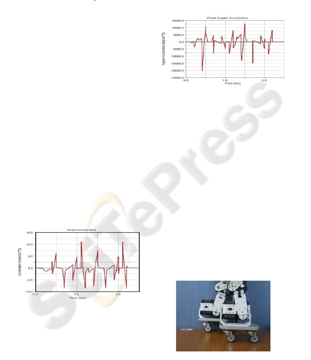
Figure 7: ADAMS Model Acceleration.
Figure 7 and figure 8 are showing the
acceleration and angular acceleration of the model
and a single wheel of the model respectively. These
plots were taken from MSC.ADAMS software.
Comparing these values to our Matlab plotting in
figure 4 and figure 5 we can see that the results in
both MSC.ADAMS simulation and our derivation of
the equations of motion agree with one another.
Both results show that as the acceleration increases
the angular acceleration on the wheels will increase
as well.
Figure 8: ADAMS Wheel Angular Acceleration.
4 CONCLUSIONS
This paper presents a simulation model with defined
motion steps to generate a human-like skating
motion. The simulation uses a robot which has two
passive wheels on each foot along the middle of the
foot. We successfully simulated the skating motion
and generated a forward motion.
We also calculated the equations of motions for
this model, and used Matlab to find a feasible value
for dependent variables. The results were compared
between the simulation and the mathematical model
successfully. Even though this was a successful
simulation, our next step will be to generate this
motion in a real humanoid that follows the model, as
can be seen in figure 9, figure 10 and figure 11.
Additionally, researching a sounder algorithm to
produce a more smooth ‘D’ shape would be
valuable. Finally, further research would be to
create a humanoid based on our model which would
have the ability to transform itself between wheeled
locomotion and leg locomotion depending on the
surface it is crossing (even or uneven).
Figure 9: Small Size Humanoid Wheels.
ICINCO 2010 - 7th International Conference on Informatics in Control, Automation and Robotics
358
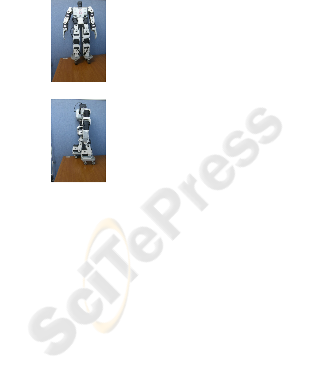
Figure 10: Small Size Humanoid Front View.
Figure 11: Small Size Humanoid Side View.
REFERENCES
Chitta S., Kumar V., 2003. Dynamics and Generation of
Gaits for a Planar Rollerblader. International
Conference of Intelligent Robots and Systems.
Endo G., Hirose S., 1999. Study on Roller-Walker
(System Integration and Basic Experiments.)
International Conference on Robotics and
Automation.
Endo G., Hirose S., 2000. Study on Roller-Walker (Multi-
mode Steering control and Self-contained
Locomotion.) International Conference on Robotics
and Automation.
Hashimoto K., Hosobata K, Sugahara Y., Mikuriya Y,
Lim H., Takanishi A., 2005. Realization by Biped
Leg-wheeled Robot of Biped Walking and Wheel-
driven Locomotion. International Conference on
Robotics and Automation.
Hirose S., Takeuchi H., 1996. Study on roller-walker
(Basic Characteristics and its Control.) International
conference on Robotics and Automotion.
Honda, ASIMO, January, 13
th
2010. The New ASIMO –
Major Features Summary. http://www.hondauk-
media.co.uk/uploads/presspacks/bf27134f6692b1c050
d8ae9c29bc21840af2a723/Major_Features_Summary.
pdf
Jo S., Chu J., Lee Y., 2008. Motion Planning for Biped
Robot with Quad Roller Skates. International
conference on Control, Automation and System.
National Research Council Special Report 286, 2006.
Tires and Passengers Vehicle Fuel Economy.
Washington D.C.
Peck William Guy , 1859. Element of Mechanics: For the
Use of Colleges, Academics and High Schools. A.S.
Barnes & Burr. New York
Ylonen S. J., Halme A. J., 2002. WorkPartner – Centaur
like Service Robot. Intl. Conference on Intelligent
Robots and Systems.
MOTION GENERATION FOR A HUMANOID ROBOT WITH INLINE-SKATE
359
