STEREO VISION BASED VEHICLE DETECTION

Benjamin Kormann, Antje Neve, Gudrun Klinker and Walter Stechele

BMW Group Research and Technology, Vehicle Sensors and Perception Systems, Hanauerstr. 46, Munich, Germany

Technische Universit

at M

unchen, Boltzmannstr. 15, Garching, Germany

Keywords:

Stereo vision, Vehicle detection, GPS evaluation.

Abstract:

This paper describes a vehicle detection method using 3D data derived from a disparity map available in real-

time. The integration of a ﬂat road model reduces the search space in all dimensions. Inclination changes

are considered for the road model update. The vehicles, modeled as a cuboid, are detected in an iterative

reﬁnement process for hypotheses generation on the 3D data. The detection of a vehicle is performed by a

mean-shift clustering of plane ﬁtted segments potentially belonging together in a ﬁrst step. In the second step

a u/v-disparity approach generates vehicle hypotheses covering differently appearing vehicles. The system

was evaluated in real-trafﬁc-scenes using a GPS system.

1 INTRODUCTION

The automobile industry has been facing many chal-

lenging tasks for years. Motor vehicle manufactur-

ers and component suppliers have constantly enriched

the driving comfort of today’s vehicles over the last

decades and have made them more secure, with appli-

cations like Damper Force Control (DFC) or Dynamic

Stability Control (DSC).

Adaptive Cruise Control (ACC) uses a typical ra-

dio detection and ranging (Radar) based driving assis-

tance system, which measures the distance and speed

obstacles by a Doppler frequency shift. Radar proved

to be a suitable sensor for applications needing dis-

tance information. Some applications like Lane De-

parture Warning or Trafﬁc Sign Detection use cam-

eras, because Radar cannot interpret visual data. Be-

cause a high number of applications per sensor is de-

sired, it is worth trying to have cameras perform ACC

by scanning and analyzing the surrounding environ-

ment.

The entire infrastructure of trafﬁc guidance is de-

signed for visual perception, and therefore it is obvi-

ous to evaluate a vision-based ACC approach. The

drawback of a single-camera system is the loss of

depth, because only a projection of the scene is cap-

tured. A stereo vision system, containing two cam-

eras, overcomes this drawback. Much like how hu-

mans who retrieve 3D information with two eyes, a

stereo machine vision can reconstruct the 3D world

with two cameras.

This work provides an analysis of whether the

higher costs of two cameras are worth the expense

compared to value that the higher number of appli-

cations the system can cover.

This paper is organized as follows: ﬁrst an

overview of previous work will be given in section 2,

then we will describe the iteratively reﬁning vehicle

detection process in section 3. Section 4 evaluates the

implemented system and provides a conclusion of this

paper.

2 PREVIOUS WORK

Bertozzi et al. perform vehicle detection on a stereo

vision-based system (Bertozzi et al., 2000). They try

to identify vehicles due to their symmetry in single

images. The symmetry is determined on horizontal

and vertical edges with a threshold. Such a symmetry

map describes the degree of symmetry by its pixel in-

tensities and the width of the symmetric object by its

spread along the ordinate. The stereo system is only

used to reﬁne the initially estimated distance of the

input images. This system does not operate on real

3D data producible by stereo systems and does not

exploit the complete stereo performance.

Foggia et al. propose a stereo vision approach

in combination with optical ﬂow to extract their own

431

Kormann B., Neve A., Klinker G. and Stechele W. (2010).

STEREO VISION BASED VEHICLE DETECTION.

In Proceedings of the International Conference on Computer Vision Theory and Applications, pages 431-438

DOI: 10.5220/0002847004310438

 SciTePress

movement (Pasquale Foggia et al., 2005). The dispar-

ity map is resampled and quantiﬁed according to the

resolution of the optical ﬂow. The displacement of

each point in the disparity map in adjacent frames can

be predicted, if the camera motion is known. In case

a point belongs to a moving object, the observed mo-

tion vector differs from the predicted and if it exceeds

a threshold, a blob detection is used to combine the

connected components. This approach was applied

to synthetic scene data generated by a rendering soft-

ware, but it doesn’t provide performance information

on vehicle detection.

Toulminet et al. extract obstacle features out of

a feature-based sparse disparity map by bidirectional

edge matching (Gwenaelle Toulminet et al., 2006).

The connected 3D points of an object in the scene

are back projected, where a connecting, depth and

uniqueness criteria is applied. A v-disparity map

in combination with a Hough transform determines

the road plane and obstacles are detected due to a

threshold comparison of the disparities with respect

to the road. Vehicle hypotheses are generated simi-

lar to (Bertozzi et al., 2000) by the generation of a

symmetry map. For each candidate a bounding box is

created by a pattern matching for the detection of the

lower vehicle part.

Obstacle detection on disparity images is pro-

posed by Huang et al. (Huang et al., 2005). They

segment the disparity image in different layered im-

ages at several disparities along with a certain offset.

The selection of the disparities is unknown a priori,

because it can slice vehicles in parts and return any

nearby merged object. Since linear relationship be-

tween the disparity and the depth doesn’t have to be

given, depending on the rectiﬁcation procedure, the

computed offset would have to be depth dependent.

Labayrade et al. perform obstacle detection on

u/v-disparity maps (Labayrade et al., 2002). They

noticed that objects expanding in viewing depth di-

rection project a linear curve, a diagonal line respec-

tively in the v-disparity image. The intersection of

this curve and vertical lines represent the tangency of

an obstacle with the road. Additionally, they adapt

the road proﬁle by an evaluation of two consecutive

v-disparity maps. The vehicle detection solely rely-

ing on u/v-disparity maps is likely to fail, because

the possible measurement failure in disparity compu-

tations is further integrated in these maps, see also

section 3.1.3.

Applications in the automotive environment de-

mand a robust and reliable rate of success in all cases.

If a million vehicles are sold in dozens of countries

every year with an installed sensor along with its ap-

plication, the environments will be dissimilar to each

Images

Hypotheses Generation

Hypotheses Veriﬁcation

Object List

PreProcessing

Reﬁnement

Hypotheses

Scene Objects

Augmentation

Figure 1: Two stage iterative reﬁnement approach.

other. Neither the shape nor the color of any appear-

ing object is completely predictable, but the applica-

tion must be self-adaptive and reliable in all situations

in the present and the future. It also may not be for-

gotten that the needed sensors must be low priced and

satisfy high quality criteria like durability, stability in

realistic temperature ranges.

3 VEHICLE DETECTION

The difﬁculty of object detection is mostly not the ob-

ject detection process itself, but rather the inﬂuence of

the environment on the appearance. In urban trafﬁc

scenarios there exist many uncertain background ob-

jects that distract the detection process from a proper

mode of operation. Additionally, the camera itself

travels through the environment, such that static ob-

jects move along the inverse direction of the camera

and objects at the same speed appear to be constant.

This work proposes a two stage iterative reﬁne-

ment for vehicle hypotheses generation. The under-

lying vehicle model taken for detection purpose is a

cubical shape contour. This approximation is suitable

for most vehicle types and is also often used for occlu-

sion handling (Pang et al., 2004; Chang et al., 2005).

Figure 1 illustrates the iterative approach, whose com-

ponents are further described in the following sec-

tions.

3.1 Hypotheses Generation

A vehicle appearance depends on its pose, as it re-

sides in the real world with respect to the camera sys-

tem. Additionally, vehicles tend to be different from

the point of view in color or shape. The complex en-

vironment complicates the vision-based recognition

process since there are many objects that are not of

interest like trees, trafﬁc signs, or bicycles which may

cause intensity variations due to occlusion and shad-

ing. Because of all these possible inﬂuences, vehicle

candidates are extracted from the image as hypothe-

VISAPP 2010 - International Conference on Computer Vision Theory and Applications

432

ses. Since vision-based vehicle detection has received

a lot of attention for trafﬁc surveys or driver assis-

tance, many methods emerged for hypothesis gener-

ation, and they can be classiﬁed into the three cate-

gories knowledge-, stereo- and ﬂow-based (Sun et al.,

2006).

This work evaluates the Standardized Stereo Ap-

proach and generates vehicle hypotheses from 3D

data retrieved by the disparity map, which is available

in real-time since its computation is implemented in

hardware. The iterative two stage model is applied to

3D data.

3.1.1 Assumption

As stated before, a vehicle is modeled as a cuboid

scalable in width, length, and height. A natural scene

may contain many objects following this model like

buildings, road side advertisement, or road signs,

which may lead to many false hypotheses. Moreover,

the search space is tremendously high if there is no

restriction on possible vehicle positions or on the ob-

ject dimension. Since all vehicles to be detected are

approximately on the same altitude with respect to the

road, the search complexity can be reduced assuming

that all four vehicle sides are orthogonal to it. This

requires a road model, which represents the actual

course of the road.

This approach uses a ﬂat road assumption, be-

cause it is sufﬁcient for most cases like urban or

highway trafﬁc (Hong Wang, 2006), (Huang et al.,

2005), (Sergiu Nedevschi et al., 2004), (Gwenaelle

Toulminet et al., 2006), Labayrade (Labayrade et al.,

2002) considers a ﬂat and non-ﬂat road geometry.

3.1.2 Stage 1 of Hypotheses Generation

In the ﬁrst hypotheses generation stage, an instance

of the cubic model must be created for each possible

vehicle candidate in the scene. Despite of the fact a

cuboid has six facets, only three of them can at most

be captured by the stereo system. It will seldom be

the case, that the front or rear, lateral and top side of

a vehicle may be visible in an image.

The Summed Absolute Differences (SAD) dispar-

ity map in ﬁgure 2(b) shows a vehicle with two visible

facets, where bright points represent small absolute

disparity values, which means the object is further

away, and dark points represent high absolute dispar-

ity values, which means the object is close by. The

white spots in the disparity map are regions out of

domain meaning that no disparity value could be es-

tablished. If not explicitly stated otherwise this work

considers large disparities as large absolute disparity

values, thus close objects.

(a) Jigsaw pieces of a vehi-

cle

(b) Vehicle boundary in dis-

parity map

Figure 2: A vehicle reassembled by its pieces of a puzzle.

Pre-selection. In a ﬁrst step the 3D data returned by

the stereo sensor must be processed to discriminate

objects from the background.

The region growing partitioning technique uses

a measure among pixels in the same neighborhood,

which tend to have similar statistical properties and

can therefore be grouped into regions. If adjacent re-

gions have signiﬁcantly different values with respect

to the characteristics on which they are compared to,

the similar interconnected pixels can reliably be re-

turned as regions.

The similarity is measured on the absolute differ-

ence of the gray values g, which represent disparity

values. The image is rastered into rectangles of size

m × n (here: 7 × 7). The values of the center points

and c

the so called seed points of two adjacent

rectangles are compared and the regions are merged

if equation (1) is satisﬁed. The threshold t

f ix

is taken

for all rectangles across the image.

|g(c

) −g(c

)| < t

f ix

(1)

This so called region growing technique is used

for segmentation on the disparity map. In this set of

regions, foreground and background assignments are

mixed. These regions will be called segments from

now on.

Filtering. First this ﬁltering step processes the seg-

ment data globally, so that all 3D point locations are

compared to the road. The street may contain irrele-

vant objects like wheel traces or green spaces on the

road side. These features can be excluded from the

3D data by a restriction on the lowest point relative

to the road proﬁle. Furthermore, a maximum height

as an upper ﬁltering bound may exclude trafﬁc signs

higher than the highest expected vehicle.

A dataset can include random measurement errors

or systematic measurement errors caused by a wrong

calibration or wrongly scaled data. The 3D data of

each segment spreads along each dimension, but es-

pecially the depth tolerance is high. A typical char-

acteristic of an outlier is the exorbitant deviation to

all other data points of the segment. Such a deviation

STEREO VISION BASED VEHICLE DETECTION

433

can statistically be expressed by the 2σ rule (Thomas

A. Runkler, 2000). A 3D point P

of a segment S is

classiﬁed as outlier, if at least one component (x, y,

z) deviates more than twice the standard deviation σ

from the mean P. The identiﬁed outliers of each seg-

ment may now be processed. Runkler proposes the re-

moval of an outlier among other approaches (Thomas

A. Runkler, 2000).

Fitting. The disparity map has now been processed

so that only those segments remain that can possibly

belong to a vehicle. The points within each segment

may never be perfectly coplanar, not even after the

previous ﬁltering step. The best solution utilizes the

linear algebra factorization Singular Value Decompo-

sition (SVD). Equation (2) shows the matrix A which

holds all m points of segment S and the vector B con-

tains the plane coefﬁcients in the linear system of

equations. If a point lies in a plane the product of

the coordinates and the plane equation must be zero.

A ·B = 0,

























= 0 (2)

The singular value decomposition of the non-

square matrix A solves the overdetermined system

of equations and returns the coefﬁcients of the ﬁtted

plane. The matrix A is an m × n matrix with m ≥ n

and can be factored to A = U DV

, where U is an

m × n matrix with orthogonal columns, D is an n × n

diagonal matrix and V is an n × n orthogonal ma-

trix (Richard Hartley and Andrew Zisserman, 2003).

The diagonal matrix D contains non-negative singu-

lar values in descending order. The column points in

V of the smallest corresponding singular value repre-

sents the solution.

The next paragraph explains how the segments are

taken together with its ﬁtted planes to merge them into

to the cubic vehicle facets.

Clustering. Although all segments have an orienta-

tion due to the ﬁtted plane and a vehicle model facet

with the same outer orientation could be instanced,

the segments cannot be merged primitively from their

normal vectors. A na

ıve combination of the segments

without any consideration of their position, orienta-

tion and density may cause false assignments and lead

to system failures.

The Mean-Shift procedure allows clustering on

high dimensional data without the knowledge of the

expected clusters and it doesn’t constrain the shape

of the clusters. Comaniciu and Meer use the mean-

shift procedure for feature space analysis (Dorin Co-

maniciu and Peter Meer, 1998), (Dorin Comaniciu

and Peter Meer, 2002). The mean-shift is formally

deﬁned as follows. The p dimensional data points

, i = 1, . . . , n ∈ R

and a multivariate kernel den-

sity estimate with the kernel K(s) in combination with

the window radius h are given, see equation (3). The

modes of the density function can be found where the

gradient becomes zero 5 f (s) = 0. The ﬁrst term of

equation (4) is proportional to the density estimate

with a radially symmetric kernel K(s) = c

k,p

k(ksk

)

and its proﬁle k, where c

k,p

ensures that K integrates

to 1. Assuming that the derivative of the kernel proﬁle

exists, the function g(s) = −k

(s) replaces the previ-

ous kernel by G(s) = c

k,p

g(ksk

f (s) =

∑

i=1



s − s



(3)

5 f (s) =

k,p

p+2

∑

i=1



s − s



· m

h,G(s)

(4)

The second term is the so called mean-shift:

h,G(s)

∑

i=1



s−s



∑

i=1



s−s



− s (5)

After the data has been standardized it can be clus-

tered by mean-shift. The approach in (Chang et al.,

2005) is based on a template matching method for a

generic vehicle, while the approach shown here fo-

cuses on a cuboid model of vehicles ﬁtted by planes.

The mean-shift algorithm is used for peak detection

in 2D score images of the matching procedure, while

here it is applied to 6D data for vehicle side candidates

retrieval.

Figure 3(b) shows the clustering result in the 3D

view. The two black points of the huge scatter cloud

on the right side represent the center of the bounding

planes of the truck visible in the disparity image in

ﬁgure 3(a).

(a) Disparity image contain-

ing a truck

(b) Black points are the clus-

tering result

Figure 3: The clustering result of all segments.

VISAPP 2010 - International Conference on Computer Vision Theory and Applications

434

Assembling. A set of planes needs to be processed

after the clustering. It depends on the position and

orientation of the planes, whether they belong to one

common vehicle or not. Since the road proﬁle is con-

sidered to ease the detection process by a restriction

of the search space, the relative height of all planes

may be evaluated prior to the assembly to exclude

non-vehicle features. The striking argument whether

two planes are candidates to be assembled is the dis-

tance of the center points. If this distance is roughly

half the width, the planes get assembled. Two planes

in 3 dimensional space intersect in a line if they aren’t

parallel. The planes π

: a

x + b

y + c

z + d

= 0

and π

: a

x + b

y + c

z + d

= 0 with (a

, b

, c

)

, b

, c

)

will intersect in a line.

All assembled planes have instanced a vehicle

model with all parameters, as there are center point,

width, height and length. All other remaining planes

that could not be merged with others are candidates

for partially visible vehicles. This missing informa-

tion must be looked up in a ratio table of common

vehicle dimensions.

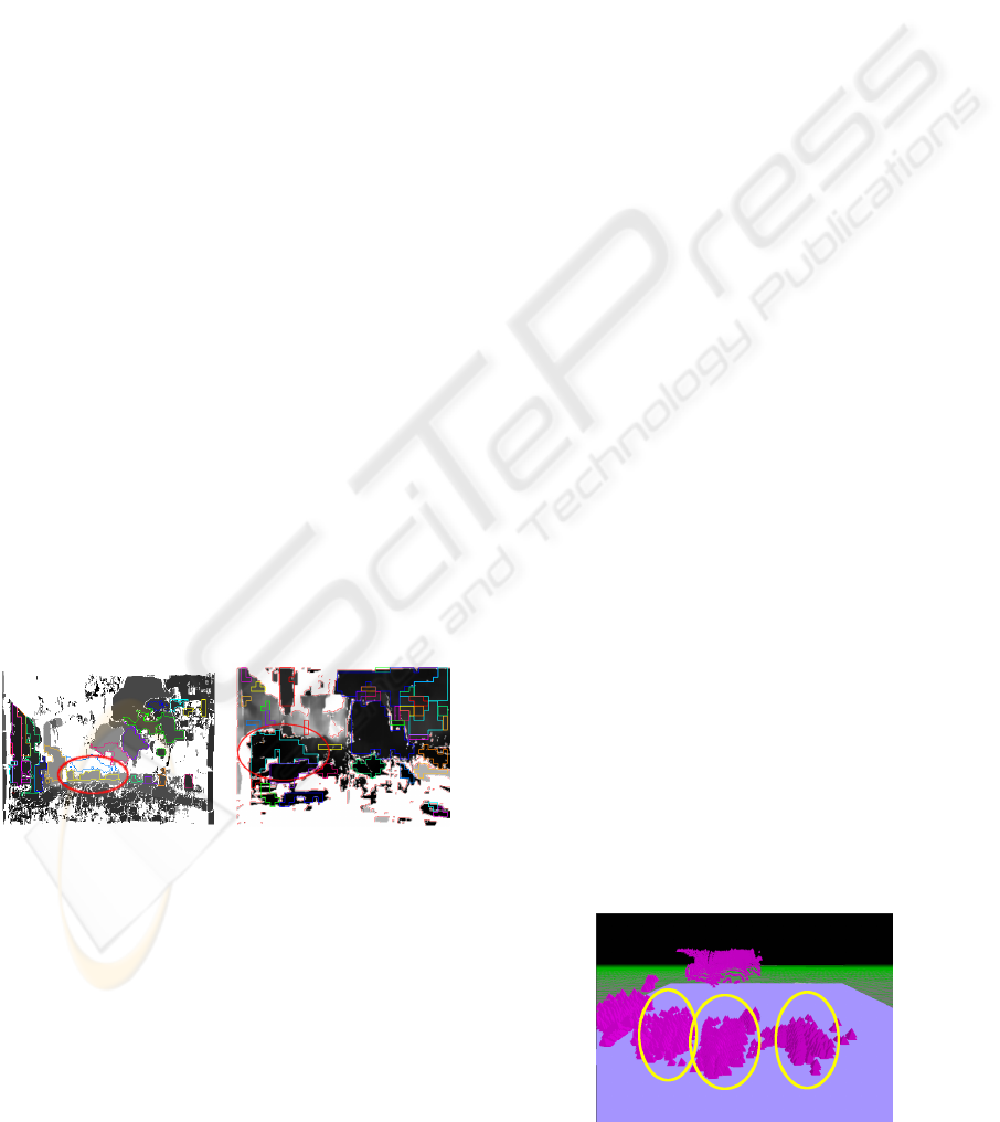
3.1.3 Stage 2 of Hypotheses Generation

In the second stage those vehicles should be identi-

ﬁed, which couldn’t be covered by the ﬁrst stage. The

quality of the result of the ﬁrst stage may be affected

negatively by the region growing response.

Figure 4(a) slightly merges three far distant vehi-

cles indicated by the yellow regions in the center of

the image surrounded by the red circle. Another neg-

ative effect of the region growing is demonstrated in

ﬁgure 4(b). The vehicle on the left side is visible from

the rear-end and the right side in the reference image.

(a) Merged regions of far

distant vehicles

(b) Two vehicle boundaries

merged as one region

Figure 4: Drawbacks of the region growing in stage 1.

U/V-Disparity. The u/v-disparity approach exploits

the information in the disparity map. V-disparity im-

ages are sometimes also used to estimate the road

proﬁle (Labayrade et al., 2002). Formally the com-

putation of the v-disparity image can be regarded

as a function H on the disparity map D such that

H(D) = D

. H accumulates the points in the disparity

map with the same disparity value d row-by-row. The

abscissa u

of a point p in the v-disparity image cor-

responds to the disparity value d

and its gray value

g(d

) := r

to the number of points with the same dis-

parity in row r:

∑

P∈D

· δ

(6)

The Kronecker delta δ

i, j

is deﬁned as follows:

i, j

(

1 for i = j

0 for i 6= j

(7)

After the disparity map has been processed for all

rows, the v-disparity image is constructed. The com-

putation of the u-disparity image is done analogously

column-wise instead of row-wise. Vertical straight

curves in the v-disparity image refer to points at the

same distance over a certain height. The upper and

lower curve delimiting points indicate a depth discon-

tinuity and may therefore represent a boundary of an

object in the image. A linear curve in the u-disparity

image utilizes the transverse depth discontinuities of

an object just as well. The intersection of the corre-

sponding back projected curve ranges deliver objects

lying frontoparallel relative to the camera. The selec-

tion of these features for vehicle detection is further

explained in the next paragraph.

Selection. Since these images localize regions in

the image whose 3D representative has a ﬁxed dis-

tance to the camera, the second stage will take care of

unidentiﬁed vehicles visible by its rear-end side. The

issue of interconnected regions in ﬁgure 4(a) due to

the satisfying similarity tolerance in the region grow-

ing process can be solved. The yellow regions sym-

bolize three far distant vehicles. Figure 5 shows the

3D view of such a situation with three spatially close

vehicles. These vehicles will appear as a linear curve

in the v-disparity image, since they are approximately

projected in the same range of rows. They will also

imply a horizontal line segment in the u-disparity im-

age, but at different frequencies, because less dispar-

ity values are present between the vehicles.

Figure 5: 3D view of interconnected vehicles.

STEREO VISION BASED VEHICLE DETECTION

435

A sophisticated way of breaking these links apart

is to declare the links at lower frequencies as outlier

with respect to the vehicle body. The detection and

removal may then be performed with the 1σ-rule.

The u/v-disparity approach is also suited well for

the second drawback of stage 1 of hypotheses gener-

ation illustrated in Figure 4(b). The disparity value

computation for the back and side plane of the ve-

hicle returned values being smaller than the region

growing tolerance, thus they got merged. Since the

u/v-disparity approach looks for frontoparallel vehi-

cle rear-end sides, both disparity patches result in dis-

tinct rows and are treated separately. Even if two

hypotheses are generated by the second stage, a sub-

sequent veriﬁcation stage will eliminate non rear-end

vehicle candidates.

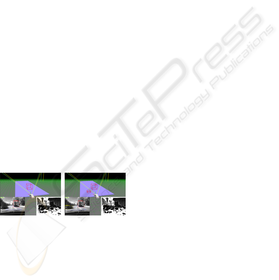
Assembling. Each rear-side vehicle candidate is

treated individually and is not merged with any other

candidate. A consideration of a remerge would have

to receive great care in order not to violate the basic

principle of this approach. Such a treatment is not

investigated in the scope of this work.

The assembly is alike to the one in stage 1. A vehi-

cle model can be instanced with the means of a lookup

table to get the length of a vehicle. This approach

tends to produce more hypotheses over the ﬁrst stage.

Thus a height restriction is taken to dump those candi-

dates that are too small to be considered as a vehicle.

Figure 6(a) shows the already veriﬁed vehicles of the

disparity map in ﬁgure 4(b) without the second stage

and ﬁgure 6(b) visualizes the result of the collabora-

tion of both stages.

(a) Vehicle detection with-

out the second stage

(b) Vehicle detection includ-

ing the second stage

Figure 6: Inﬂuence of the second stage on vehicle detection.

4 EVALUATION

The proposed technique has been tested with two dif-

ferent stereo vision systems on a Desktop PC with

3.2 GHz and 1 GB RAM in the debug environment

with visual output. The intrinsic parameters of the

camera systems A and B (different manufacturers, dif-

ferent baselines) as well as the intrinsic and extrin-

sic parameters of the binocular system must be de-

rived, in order to transform input images geomet-

rically such that proportions or real world objects

are preserved. The Marquardt-Levenberg (Stephan

Lanser et al., 1995) procedure solves the non-linear

minimization problem:

d(p) =

∑

j=1

∑

i=1

k ˆm

i, j

− π(m

, p)k

−→ min (8)

After the intrinsic camera parameters of both cameras

are determined, the 6D outer orientation of both cam-

eras with respect to a calibration table visible in both

views can be exploited to derive the relative pose of

the cameras to each other by a transitive closure. The

retrieved parameter set calibrates the sensor stereo-

scopically.

4.1 Test Setup

The Leica GPS-1200 system enables the acquisition

of object position data relative to each other at a pre-

cision at centimeter scale (Vogel, 2007), (Vogel K.,

2008). For the test scenario two vehicles equipped

with the Leica system were used. The host vehi-

cle is a BMW 5-series, which has all the sensors for

stereo data acquisition, CAN data registration and ref-

erence data integration into the developer framework

installed.

4.2 Results

The sequences cover realistic trafﬁc scenarios like a

laterally shifted vehicle following, braking maneuver

down to stop with a subsequent acceleration and driv-

ing at an adequate distance.

The red graph in ﬁgure 7(a) shows the unﬁltered

Leica reference depth data overlayed over the green

graph stating the unﬁltered stereo sensor depth data.

Sometimes the reference data oscillates strongly like

in the ﬁrst 250 frames. This is an indicator, that the

correction data quality wasn’t sufﬁcient to enable a

precise position measurement. But from that frame

on the graph characteristics looks fairly steady. The

green stereo sensor trajectory has a smooth run over

time, since the 3D data is processed by all the steps

in the iterative reﬁnement for vehicle detection ex-

plained in this chapter.

In the second sequence there is no stop and go

trafﬁc scenario, but rather a speedup of the target ve-

hicle running ahead up to a higher distance. The tar-

get vehicle longitudinal distance is stated at 26.381m

by the Leica reference system, whereas the distanced

measured and processed by the stereo sensor with

VISAPP 2010 - International Conference on Computer Vision Theory and Applications

436

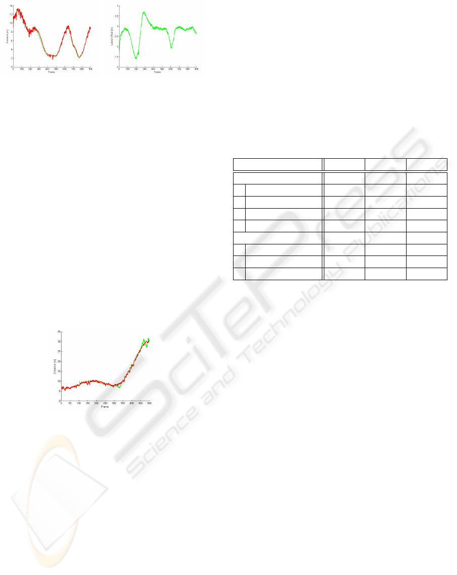
(a) Unﬁltered depth distance

in RDS 1

(b) Unﬁltered lateral shift

measured by stereo sensor in

RDS 1

Figure 7: Unﬁltered distances of target vehicle.

its algorithms comes to 25.711m. This deviation is

still within the theoretical depth resolution given by

stereo conﬁguration parameters. The total depth per-

formance comparison is stated in the diagrams in ﬁg-

ure 8. These results clearly show a good distance

performance of the stereo sensor, even at higher dis-

tances. These results clearly show a good distance

performance of the stereo sensor, even at higher dis-

tances. The theoretical depth resolution at 30m is ap-

proximately 95cm already and since the target vehicle

appears with less pixels and therefore wider 3D data

point positions after reconstruction the resulting devi-

ation of depth computation is the logical closure. The

gap between both trajectories around frame 330 might

be caused by a little latency of the road model update.

Figure 8: Unﬁltered depth distance of target vehicle in RDS

Table 1 shows the time complexity of the pro-

posed algorithms. The statistical evaluation was ap-

plied to the execution times of multiple sequences

and calibration sets. The vehicle detection algorithms

were tested on a single processor desktop computer

with 3.2 GHz and 1 GB RAM in the debug environ-

ment with visual output. Therefore none of the im-

plemented algorithms was executed at full speed, be-

cause of an additional status output in all stages to

observe the correctness of operation. If such a sys-

tem was implemented on automotive compliant hard-

ware with e.g. multiple cores, some computations

like plane ﬁtting, clustering, u/v-disparity or symme-

try map could be performed in a fraction of the stated

time. The remarkable time needed for u/v dispar-

ity computation could also be reduced if it was im-

plemented in hardware. The desktop implementa-

tion of it was not focused for time efﬁcient compu-

tation, rather for easy modiﬁable testing variations.

The assembling strategy in the ﬁrst stage has in the

worst case of n read-end planes and m side planes

m × n comparisons and thus the processing time has a

huge deviation between the minimum and maximum.

Given the u/v-disparity could be retrieved at image

acquisition time like the disparity image itself, the av-

erage processing time of the desktop implementation

comes to approximately 390ms.

Table 1: Temporal complexity of vehicle detection.

Processing Step t

min

max

mean

Stage 1 230 ms 390 ms 285 ms

Region growing 130 ms 180 ms 150 ms

Plane Fitting 55 ms 95 ms 70 ms

Clustering 10 ms 25 ms 15 ms

Assembling 35 ms 90 ms 50 ms

Stage 2 188 ms 348 ms 250 ms

u/v Disparity 170 ms 305 ms 220 ms

Selection 3 ms 8 ms 5 ms

Assembling 15 ms 35 ms 25 ms

5 CONCLUSIONS

This approach has shown that vehicle detection can

be performed accurately with a stereo vision sensor

in the challenging automotive environment. The ﬁrst

stage of the iterative reﬁnement approach in vehicle

detection allows the recognition of vehicles with the

underlying cubic model in most cases and works best

for vehicles being spatially well covered. The con-

sidered ﬂat road model eliminates road curbs and ob-

jects higher than vehicles like the ceiling of a tunnel or

direction signs, which enhances the recognition pro-

cess due to a scene simpliﬁcation. The plane ﬁtting on

each segment returned by the region growing proce-

dure on the 3D data computes an important attribute

for later clustering to vehicle plane candidates. It was

unsheathed that planes ﬁtted into those segments be-

longing to background objects like limbs and leaves

of trees have a normal vector pointing upwards with

respect to the road proﬁle and can therefor be masked

out. The 6D mean-shift clustering process containing

3D position data of all segments and their unit normal

vectors merges the segments belonging to the same

vehicle efﬁciently and robust for the vehicle assem-

bly according to the cubical model.

The second stage of the iterative reﬁnement local-

izes vehicles visible from the rear-end with the means

of u/v disparity images. This approach recognizes ve-

STEREO VISION BASED VEHICLE DETECTION

437

hicles being spatially close together even if the corre-

sponding regions in the disparity map are intercon-

nected. The method breaks such a horizontal link

apart and present vehicles are extracted in combina-

tion with the road proﬁle. The combination of these

two iterative stages has shown to be an excellent de-

tection technique.

These algorithms were tested on both stereo vi-

sion systems in urban trafﬁc and autobahn scenarios.

The stereo sensor B has shown a better performance,

which goes back to the larger baseline. The smaller

baseline of the system A would demand a more ag-

gressive ﬁltering stage for outlier removal due to the

depth resolution of the stereo conﬁguration. This

eliminates important feature points which makes ve-

hicle detection unreliable for the automotive usage.

The baseline of the system B is variable and was cho-

sen as twice the size of system A. This enabled a reli-

able detection and depth reconstruction of up to 30m

and vehicles could even be identiﬁed at higher dis-

tances, but with inaccurate dimensions. The vehicle

recognition quality was steady over the speed range

30 km/h - 130 km/h. This approach produces suitable

output for a vision-based ACC application. Parts of

this article have also been published as part of (Neve,

2009).

REFERENCES

Bertozzi, M., Broggi, A., Fascioli, A., and Nichele, S.

(2000). Stereo vision-based vehicle detection.

Chang, P., Hirvoven, D., Camus, T., and Southall, B.

(2005). Stereo-Based Object Detection, Classiﬁcation

and Quanititative Evaluation with Automotive Appli-

cations. In Proceedings of the 2005 IEEE Computer

Science Conference on Computer Vision and Pattern

Recognition (CVPR’05).

Dorin Comaniciu and Peter Meer (1998). Distribution Free

Decomposition of Multivariate Data. In SSPR/SPR,

pages 602–610.

Dorin Comaniciu and Peter Meer (2002). Mean Shift:

A Robust Approach Toward Feature Space Analysis.

IEEE Transactions on Pattern Analysis and Machine

Intelligence, 24:603–619.

Gwenaelle Toulminet, Massimo Bertozzi, Stephane Mous-

set, Abdelaziz Bensrhair, and Alberto Broggi (2006).

Vehicle detection by means of stereo vision-based ob-

stacles features extraction and monocular pattern anal-

ysis. In Image Processing, IEEE Transactions on, vol-

ume 15, pages 2364– 2375.

Hong Wang, Qiang Chen, W. C. (2006). Shape-based

Pedestrian/Bicyclist Detection via Onboard Stereo Vi-

sion. In Computational Engineering in Systems Ap-

plications, IMACS Multiconference on, pages 1776–

1780, Beijing, China.

Huang, Y., Fu, S., and Thompson, C. (2005).

Stereovision-Based Object Segmentation for Au-

tomotive Applications. EURASIP Journal on

Applied Signal Processing, 2005(14):2322–2329.

doi:10.1155/ASP.2005.2322.

Labayrade, R., Aubert, D., and Tarel, J.-P. (2002). Real

Time Obstacle Detection on Non Flat Road Geom-

etry through ‘V-Disparity’ Representation. In Pro-

ceedings of IEEE Intelligent Vehicle Symposium, Ver-

sailles, France.

Neve, A. (2009). 3D Object Detection for Driver Assistance

Systems in Vehicles. PhD thesis, Technische Universi-

taet Muenchen.

Pang, C., Lam, W., and Yung, N. (2004). A novel method

for resolving vehicle occlusion in a monocular trafﬁc-

image sequence. In Intelligent Transportation Sys-

tems, IEEE Transactions, volume 5, pages 129 – 141.

Pasquale Foggia, Alessandro Limongiello, and Mario

Vento (2005). A Real-Time Stereo-Vision System For

Moving Object and Obstacle Detection in AVG and

AMR Applications. In CAMP, pages 58–63.

Richard Hartley and Andrew Zisserman (2003). Multiple

View Geometry in Computer Vision. Cambridge Uni-

versity Press.

Sergiu Nedevschi, Radu Danescu, Dan Frentiu, Tiberiu

Marita, Florin Oniga, Ciprian Pocol, Rolf Schmidt,

and Thorsten Graf (2004). High accuracy stereo vi-

sion system for far distance obstacle detection. In In-

telligent Vehicles Symposium, 2004 IEEE, pages 292

– 297.

Stephan Lanser, Christoph Zierl, and Roland Beutlhauser

(1995). Multibildkalibrierung einer CCD-Kamera.

Technical report, Technische Universitt Mnchen.

Sun, Z., Bebis, G., and Miller, R. (2006). on-road vehicle

detection using optical sensors: A review. In IEEE

Transactions on pattern analysis and machine intelli-

gence, volume 28.

Thomas A. Runkler (2000). Information Mining. Vieweg.

Vogel, K. (2007). High-accuracy reference data acquisition

for evaluation of active safety systems by means of a

rtk-gnss-surveying system. In Proceedings of the 6th

European Congress and Exhibition on ITS, Aalborg.

Denmark.

Vogel K., Schwarz D., W. C. (2008). Reference maps of

adas scenarios by application of a rtk-gnss system.

In Proceedings 7th European Congress and Exhibi-

tion on Intelligent Transport Systems and Services,

Geneva. Switzerland.

VISAPP 2010 - International Conference on Computer Vision Theory and Applications

438