LOCAL SEGMENTATION BY LARGE SCALE HYPOTHESIS

TESTING

Segmentation as Outlier Detection

Sune Darkner, Anders B. Dahl, Rasmus Larsen

DTU Informatics, Technical University of Denmark, Richard Petersens plads, Kgs. Lyngby, Denmark

Arnold Skimminge, Ellen Garde, Gunhild Waldemar

DRCMR, Copenhagen University Hospital Hvidovre, Kettegaard Alle 30, DK 2650 Hvidovre, Denmark

Memory Disorders Research Group, Department of Neurology, Copenhagen University Hospital, Copenhagen, Denmark

Keywords:

Segmentation, Outlier detection, Large scale hypothesis testing, Locally adjusted threshold.

Abstract:

We propose a novel and efﬁcient way of performing local image segmentation. For many applications a thresh-

old of pixel intensities is sufﬁcient. However, determining the appropriate threshold value poses a challenge. In

cases with large global intensity variation the threshold value has to be adapted locally. We propose a method

based on large scale hypothesis testing with a consistent method for selecting an appropriate threshold for the

given data. By estimating the prominent distribution we characterize the segment of interest as a set of outliers

or the distribution it self. Thus, we can calculate a probability based on the estimated densities of outliers

actually being outliers using the false discovery rate (FDR). Because the method relies on local information it

is very robust to changes in lighting conditions and shadowing effects. The method is applied to endoscopic

images of small particles submerged in ﬂuid captured through a microscope and we show how the method can

handle transparent particles with signiﬁcant glare point. The method generalizes to other problems. This is

illustrated by applying the method to camera calibration images and MRI of the midsagittal plane for gray and

white matter separation and segmentation of the corpus callosum. Comparing this segmentation method with

manual corpus callosum segmentation an average dice score of 0.88 is obtained across 40 images.

1 INTRODUCTION

We present a novel way of performing binary seg-

mentation of images with large global variations. In

many segmentation problems such as global changes

in illumination, shadows, or background variations, a

global threshold is not a feasible solution. Variations

in pixel intensities can result in large segmentation er-

rors if one global threshold value is applied. As a

consequence the threshold has to be locally adapted.

Another problem is the dominating backgroundinten-

sities, which makes typical histogram based methods

like histogram clustering (Otsu, 1975) inappropriate.

We propose a method based on the assumption

that a local threshold exists, which will separate the

segment of interest from the background. We present

a well deﬁned way of selecting the appropriate thresh-

old value given the observations based on a large scale

hypothesis test and experimentally show that this as-

sumption is appropriate for many real segmentation

problems.

2 PREVIOUS WORK

Segmentation is a widely used technique in com-

puter vision for identifying regions of interest. Basic

threshold is a simple, very robust and fast approach

for performing segmentation. It is applicable for a

wide range of segmentation problems where regions

of interest have intensity levels which differers from

the remainder of the scene. Many techniques have

been developed for identiﬁcation of suitable thresh-

old.(Sezgin and Sankur,2004) givesan overview. The

simplest approach is to perform a global threshold for

the whole image e.g. based on the shape of the in-

tensity histogram (Sezan, 1990), applying a Gaussian

215

Darkner S., B. Dahl A., Larsen R., Skimminge A., Garde E. and Waldemar G. (2010).

LOCAL SEGMENTATION BY LARGE SCALE HYPOTHESIS TESTING - Segmentation as Outlier Detection.

In Proceedings of the International Conference on Computer Vision Theory and Applications, pages 215-220

DOI: 10.5220/0002845402150220

 SciTePress

mixture model (Hastie et al., 2001) or by performing

clustering (Otsu, 1975). Local methods have an adap-

tive threshold, which varies across the image. As a

result the local methods are suited for images with

global intensity variations (Stockman and Shapiro,

2001).

Images with regions of interest taking up a small

proportion of the image poses a challenge. Histogram

shape or clustering methods will be inadequate for

ﬁnding a good threshold since the regions of inter-

est will almost invisible in the histogram. (Ng, 2006)

suggested a threshold at a valley in the histogram

while maximizing the between segment variation sim-

ilar to Outss method (Otsu, 1975). This requires a

two-peaked distribution of the histogram, which lim-

its the applicability of the method.

Our method provides a good solution to a wider

class of intensity distribution. It can be applied both

as a global and local segmentation method which

makes it very ﬂexible. Our approach is based on the

assumption of a given intensity distribution that can

be estimated from the observed distribution. For each

intensity value there is a probability of belonging to

this distribution, which can be compared to the ac-

tual observed distribution. The difference between

the expected distribution and the observed can be in-

terpreted as false discoveries used for identifying the

threshold value. This idea originates from (Efron,

2004), who used it for identifying observations of in-

terest in genome responses.(Darkner et al., 2007) Ap-

plied it for shape analysis.

The rest of the paper is organized as follows. First

we describe the details of our method, and following

that we describe and discuss our experiments, and ﬁ-

nally we conclude our work.

3 LARGE SCALE HYPOTHESIS

TESTING

The point of large-scale testing is to identify a small

percentage of interesting cases that deserve further

investigation using parametric modeling. The prob-

lem is that a part of the interesting observations may

be extracted, but if more are wanted then also unac-

ceptably many false discoveries are identiﬁed (Efron,

2004). A major point of employing large-scale esti-

mation methods is that they facilitate the estimation

of the empirical null density rather than using the the-

oretical density. The empirical null may be consid-

erably more dispersed than the usual theoretical null

distribution. Besides from the selection of the non-

null cases (the selection problem) large-scale testing

also provides information of measuring the effective-

ness of the test procedure (estimation problem). In

this paper we employ both measures to separate the

particles from the background transform calibration

images into binary images, segment the corpus cal-

losum and separate white and gray matter in brain

images. Simultaneous hypothesis testing is founded

on a set of N null hypotheses {H

}

i=1

, test statistics

which are possibly not independent. {Y

}

i=1

and their

associated p-values { P

}

i=1

deﬁning how strongly the

observed value of Y

contradicts H

3.1 False Discovery Rate

In this paper we assume the N cases are divided into

two classes, Null and non-null occurring with prior

probabilities p

and p

= 1− p

. We denote the den-

sity of the test statistics given its class f

(z) and f

(z)

(null or non-null respectively). False discovery rate

(FDR) methods are central to some largescale method

and is employed here. It is typical to consider the ac-

tual distribution as a mixture of outcomes under the

null and alternative hypotheses. Assumptions about

the alternative hypothesis may be required. The sub-

densities

(z) = p

(z) , f

(z) = p

(z) (1)

and mixture density

f(z) = f

(z) + f

(z) (2)

leads directly to the local false discovery rate:

fdr(z) ≡ P(null|z

= z)

= p

(z)/ f(z) = f

(z)/ f(z) (3)

The FDR describes the expected proportion of false

positive results among all rejected null hypotheses

and guarantees that the fraction of the number of false

positives over the number of tests in which the null

hypothesis was rejected (Efron, 2004). Figure 1 and

2 illustrates the fundamentals of the approach.

For segmentation of particles the hypothesis test

is used to ﬁnd pixels that are a part of a segment i.e.

observations that deviates signiﬁcantly from the av-

erage local background. We use large-scale testing

to estimate the empirical null hypothesis for a given

region assuming the pixel values follows some nor-

mal distribution. It is convenient to consider z

−1

), i = {1...N} where Φ is the standard nor-

mal cdf and z

∼ N(0,1). Estimates of the pixel er-

ror and conﬁdence bounds can be mapped to N(0,1)

through Φ. As an example of prior information for

particles we see that the background has higher pixel

intensities than the particles. The background will

therefor be the highest and largest distribution. This

can be used to get a better empirical estimate of of the

null hypothesis.

VISAPP 2010 - International Conference on Computer Vision Theory and Applications

216

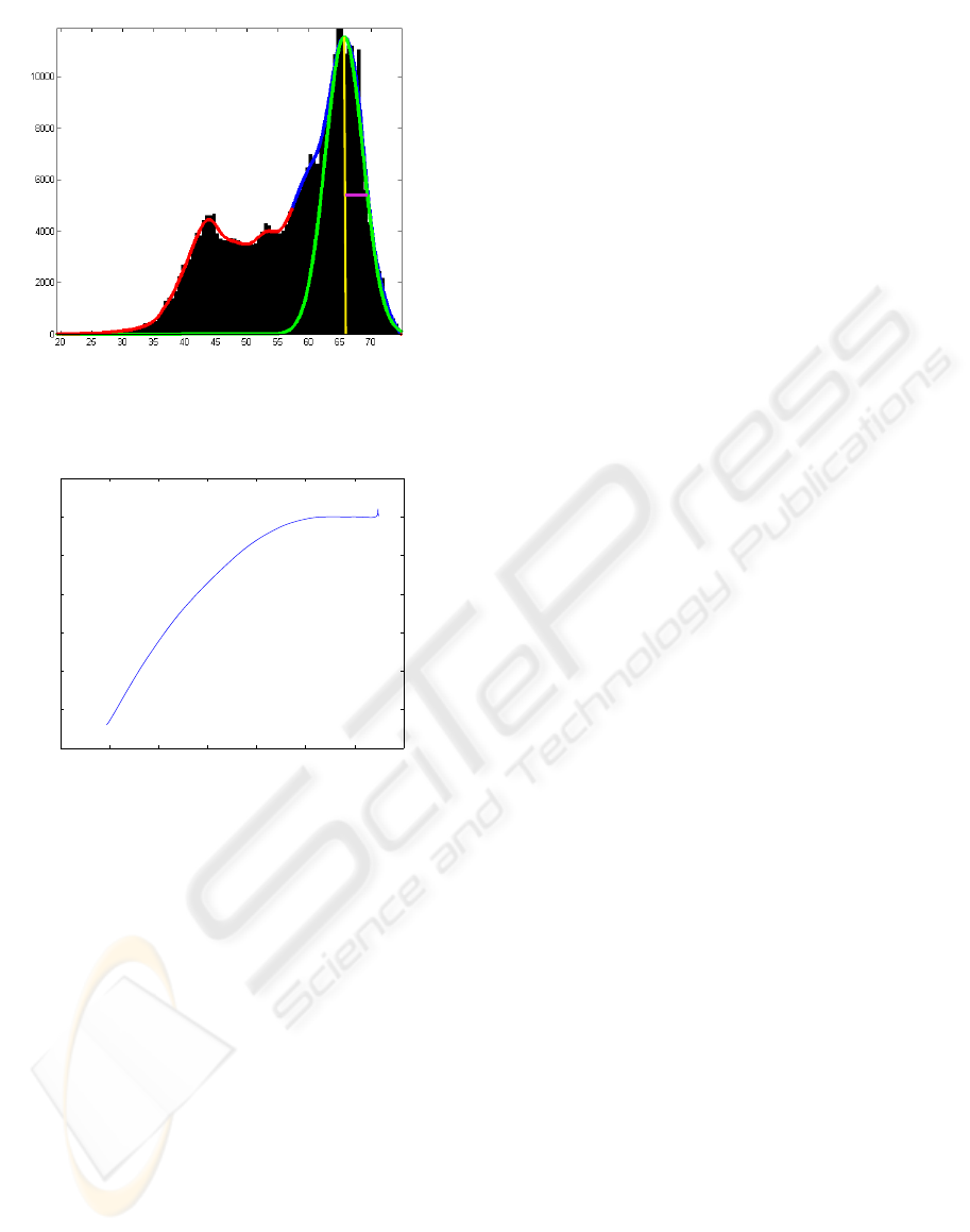
Figure 1: The graphical presentation of large scale hypoth-

esis test. The red and blue curve is f(z), the green is the pdf

of the estimated null hypothesis f

(z) where the yellow is

the mean and the purple is the half width half maximum.

10 20 30 40 50 60 70 80

−120

−100

−80

−60

−40

−20

log(FDR)

Intensity

Figure 2: The corresponding logarithm of FDR for Figure

3.2 Estimation of H

Assuming that the prominent distribution follows a

normal distribution we are able to estimate H

. Thus

for the estimation we choose an appropriate resolu-

tion and map all value into the histogram. This forms

our joint distribution f(z) to which we then ﬁt a spline

with appropriate smoothness for an approximation of

the joint distribution. We can then identify the ﬁrst

large peak as the mean value of f

(z) and use half

width, half maximum to estimate the standard devi-

ation i.e. the maximum peak of f(z) and half of the

width (see Figure 1). The obvious choice would be

full width half maximum, however there is a blending

of in the joint distribution of f

(z) and f

(z) which

gives a thicker tail towards lower intensity values and

a much more conservative estimate of the standard de-

viation (see Figure 1). The estimation of f

(z) is a

good place to apply prior knowledge of the distribu-

tions such as ordering etc.

3.3 Parameters and Their

Interpretation

In practice several parameter have to be selected. The

ﬁrst is the level at which we are willing to accept false

positives which is the an expression of the certainty

that a given observation is signiﬁcantly different from

. This does not in anyway tell us that the class is a

certain kind of tissue or particle, only that this is with

certainty p different from the null distribution thus the

observation is an outlier.

The testing area has to be selected. This criteria is

mainly driven by the object in question and the back-

ground. Sufﬁcient information about the distribution

of the object and background must be present. The

spatial sampling density has to be selected as well.

In all experiments in this paper we have up-sampled

the image by a factor of 10-100 which also yields an

equal sub-pixel resolution of the method. Usually the

test is based on 10

− 10

samples and in a 100 bin

histogram which ensures smooth estimate of f(z) and

enough resolution for gray values. In practice f(z)

is approximated by a spline thus the smoothness has

to be selected for good estimation of f

(z) and can

compensate for low number of sample.

4 EXPERIMENTS

We have applied the method to 3 sets of data. Small

particles obtained with high magniﬁcation, 2D slices

of brain MRI for segmentation of the Corpus Callo-

sum and a standard checker board for image calibra-

tion with highly varying intensity values. These 3 di-

verse applications show the versatility of this simple

but robust method. For all examples we have shown

the sampling area in the sampling resolution for both

segmentation and object.

4.1 Particles

For characterization of powders, droplets etc the size

and shape of the objects are very important. In or-

der to do a good classiﬁcation the particles need to be

found and properly segmented. The method is well

suited for images where the light source changes in

intensity and distribution locally (e.g. shadows) and

globally (e.g. illumination) from frame to frame in

a series of images, cases where robust estimate for

background removal can be difﬁcult to obtain. In ad-

dition some particles may partially shadow other par-

ticles thus making the global background removal in-

capable of segmenting the particle in question. The

method has been tested on 3 types of particle images.

LOCAL SEGMENTATION BY LARGE SCALE HYPOTHESIS TESTING - Segmentation as Outlier Detection

217

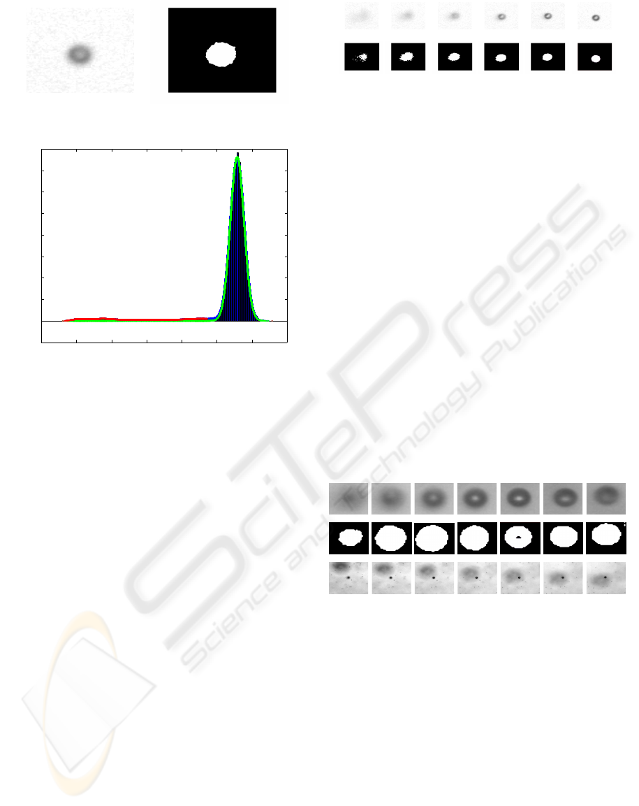
(a) The particle (b) The segmentation

100 120 140 160 180 200 220 240

−1000

1000

2000

3000

4000

5000

6000

7000

8000

Figure 3: A typical segmentation and the corresponding his-

togram. The green line in the histogram is the estimated

and the red line indicates outlier with the fdr=0.0001

The histogram clearly show how well our assumption of the

background following a normal distribution holds. The out-

lier are the particle we segmenting.

A set of LED back lit particles suspended between

2 sheets of glass with varying distance to the focus

plane . A tracking scenario with time series of cali-

brated particles suspended in water and laser back lit

non-uniform particles suspended in water.

4.1.1 Fixed Particle

We have applied the method to the 25 µ m particles

suspended in water between two sheets of glass in

with different distances to the focal plane. Figure 4

show a 25 µ m particle at 6 distances to the focal

plane. This experiment illustrates the sensitivity of

the method, where even vaguely visible particles can

be segmented without parameter tuning. The thresh-

old was selected on the criteria that the possibility of

a false positive should be less than 0.01%, the size of

the window is 40× 40 and the sampling resolution in

each direction is 0.1 pixel.

Figure 4: The images show the particle at 6 different dis-

tances to the focal plane, with the las image being of the

particle in focus. Below are the segmentations of each od

the images in the same order. The images show that the par-

ticle can be segmented even if the signal is very vague and

the glare point is correctly classiﬁed as a part of the particle.

4.1.2 Shadowing Effect

We have preprocessed all images with multi scale

blob detection (Bretzner and Lindeberg, 1998) such

that we have rough estimate of the size and location

of the blobs. This is sufﬁcient to perform the segmen-

tation. The data consists of movie sequences obtained

with 5 times magniﬁcation of semi transparent parti-

cles of 100, 50, 25 and 5 µm in a water solution and

used for illustration of handling of shadowing effects

without change to the parameters of the algorithm.

Figure 5 show a segmentation performed over sev-

eral frames where a larger particle passes in the back-

ground creating a shadowing effect. The example il-

lustrates how the methods can handle changes in the

illumination without failure. The threshold was se-

lected with p = 0.0001, windowsize of 20× 20 pixel

with a sampling resolution of 0.1 pixel.

Figure 5: The ﬁgure show a segmentation performed with

the same parameters on the same object subject to changing

shadowing effect caused by a large particle passing in the

background.

4.1.3 Real Particles

To show how the method handles real world data we

have segmented some particles of some material sam-

ples from the industry. Figure 6 and 7 show two

small examples of such particles. The segmentation

is very good due to the locally very uniform back-

ground, making the distribution of peaked and narrow

i.e. a small standard deviation. Glare points are also

handled very well but there is naturally enough a band

around the glare point where the particle is misclassi-

ﬁed. This is due to the fact that the method is just a

simple threshold without any spatial prior. These gaps

VISAPP 2010 - International Conference on Computer Vision Theory and Applications

218

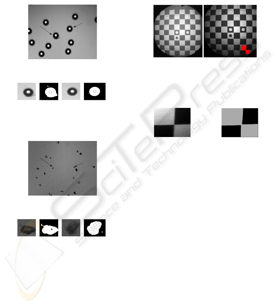
can be handled by applying an appropriate post pro-

cessing step. The results in ﬁgure 6 was made with

p = 0.0001 and a window of 200× 200 with a sam-

pling resolution of 0.3 pixels and the results in ﬁgure

7 with a window of 100× 100 same p and same reso-

lution.

(a) The original image

Figure 6: The ﬁgure show some real world samples. The

ﬁgure show that the segmentation the glare points is han-

dled very well. The small ’gap’ can be ﬁxed by a simple

morphological operation.

(a) The original image

Figure 7: Some crystal like particles are shown in the ﬁgure.

In spite of the relative low difference between background

and object and the fact that the samples are semi transparant,

the segmentation is good. Even small ones are handled to-

gether with the large ones.

4.2 Calibration Images

We also present some results on calibration images.

When using a well known structure as the checker-

board for calibration it is important to exactly locate

the corner of the squares i.e. by morphological opera-

tions on a segmented image. The proposed method

delivers very good segmentation and it is expected

that it can be used to derive the exact sub-pixel po-

sition of the corners creating a robust foundation for

image calibration. Figure 8 and 9 show the results of

the segmentation. The results in Figure 9 was made

with p = 0.0001 and a window of 100 × 100 with a

sampling resolution of 0.3 pixels.

(a) The calibration

image

(b) The calibration im-

age with the segmenta-

tion marked

Figure 8: The original calibration image. As can be seen

the intensities varies signiﬁcantly with the highest values at

the center and decaying radially.

(a) Segmented image

part

(b) Segmentation

Figure 9: The changes in gray scale values are handled quite

nicely, but causes the little gap between the two black cor-

ners in the segmentation. This can be close with morpho-

logical operations.

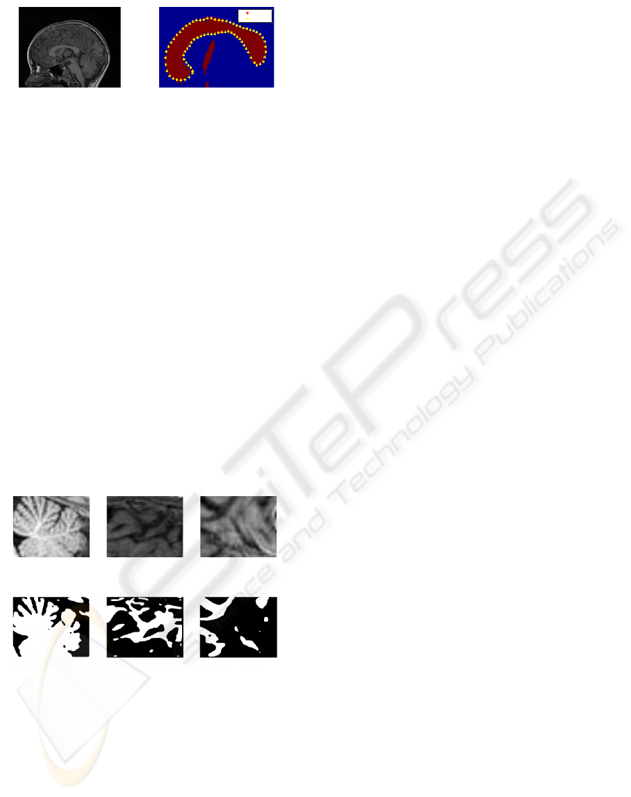
4.3 MRI

To illustrate the method on another modality, we have

applied the method to MRI scans of the human human

brain, more precisely the midsagittal plane that con-

tain the corpus corpus callosum (see Figure 10(a)).

The method has applied to white and gray matter

segmentation and segmentation of the corpus callo-

sum. In the latter case we have a manually segmented

ground truth, thus we can compute the segmentation

error via the Dice coefﬁcient (Sørensen, 1948). The

results in Figure 10 was made with p = 0.01 and a

window of 60× 80 with a sampling resolution of 0.1

pixels.

Across 40 subject with their Corpus Callosum

segmented with the AAM (Ryberg et al., 2006) and

manually corrected we found that local segmentation

through large scale hypothesis testing gave an aver-

age Dice coefﬁcient of 0.856 with a standard devia-

tion of 0.034. The Corpus Callosum was extracted in

the same hypothesis test, however if we use the local

LOCAL SEGMENTATION BY LARGE SCALE HYPOTHESIS TESTING - Segmentation as Outlier Detection

219

(a) MRI

AAM

Manual

(b) segmentation

Figure 10: (a)The midsagittal slice from an MRI of a head.

(b) This ﬁgure show the result of the segmentation of ﬁg

10(a) using the method proposed in this paper. The red dots

are the segmentation achieved by the AAM and the yellow

the manual segmentation. The read part of the image is the

segmentation with the our method. This result show how

efﬁcient this algorithm is for local segmentation.

property and us a smaller window, outliers become

more signiﬁcant and we get better segmentation. By

switching to a more local neighborhood we get a im-

provement of almost 3% to 0.880 and the difference

is very signiﬁcant (p << 0.01) using a paired t-test.

As a last test we separated the white and gray mat-

ter. The results are a little greedy, some gray matter is

classiﬁed as white matter. This is due to the fact that

the two density functions are somewhat overlapping

and that the dark regions actually is a 3 class segmen-

tation problem making it non-binary. Some improve-

ment can be obtained by adjusting the window size

and the p-value. The results in ﬁgure 11 were made

with p = 0.01 and a window of 40 × 40 with a sam-

pling resolution of 0.1 pixels.

(a) Image (b) Image (c) Image

(d) segmentation (e) segmentation (f) segmentation

Figure 11: Some results on segmenting the white matter.

The results are a little greedy including some gray matter.

5 SUMMARY AND

CONCLUSIONS

We have presented a local adaptive method for binary

segmentation. The methods has successfully been

tested on particle images for particle segmentation,

calibration images and and midsagittal slices of MRI

for segmentation of corpus callosum and gray mat-

ter white matter segmentation. The method is very

robust with respect to changes in intensity across the

image and statistically characterizes the resulting seg-

mentation. We have shown that compared to manual

segmentation of the Corpus Callosum we can achieve

a dice coefﬁcient of 0.88 on using a mosaic of 5

patches. The method is directly extendable to 3D,

other types of distribution. The hypothesis test and

FDR should be extended to higher dimensions that

the one dimensional case discussed here and tested on

several other types of images. furthermore the algo-

rithm should be implemented such that it can handle

multiple classes and segment a whole image at once.

REFERENCES

Bretzner, L. and Lindeberg, T. (1998). Feature tracking with

automatic selection of spatial scales. Computer Vision

and Image Understanding, 71(3):385–392.

Darkner, S., Paulsen, R. R., and Larsen, R. (2007). Analy-

sis of deformation of the human ear and canal caused

by mandibular movement. In Medical Image Com-

puting and Computer Assisted Intervention MICCAI

2007, pages 801–8, B. Brisbane, Australia, Springer

Lecture Notes.

Efron, B. (2004). Large-scale simultaneous hypothesis test-

ing: the choice of a null hypothesis. Journal of the

American Statistical Association, 99(465):96–104.

Hastie, T., Tibshirani, R., and Friedman, J. (2001). The Ele-

ments of Statistical Learning: Data Mining, Inference,

and Prediction. Springer-Verlag.

Ng, H. (2006). Automatic thresholding for defect detection.

Pattern Recognition Letters, 27(14):1644–1649.

Otsu, N. (1975). A threshold selection method from gray-

level histograms. Automatica, 11:285–296.

Ryberg, C., Stegmann, M. B., Sj¨ostrand, K., Rostrup, E.,

Barkhof, F., Fazekas, F., and Waldemar, G. (2006).

Corpus callosum partitioning schemes and their effect

on callosal morphometry.

Sezan, M. (1990). A peak detection algorithm and its

application to histogram-based image data reduction.

Computer Vision, Graphics, and Image Processing,

49(1):51.

Sezgin, M. and Sankur, B. (2004). Survey over image

thresholding techniques and quantitative performance

evaluation. Journal of Electronic Imaging, 13(1):146–

168.

Sørensen, T. (1948). A method of establishing groups of

equal amplitude in plant sociology based on similarity

of species content and its application to analyses of the

vegetation on Danish commons. Biologiske Skrifter,

(5):1–34.

Stockman, G. and Shapiro, L. (2001). Computer Vision.

Prentice Hall PTR, Upper Saddle River, NJ, USA.

VISAPP 2010 - International Conference on Computer Vision Theory and Applications

220