CLASSIFICATION OF CHALLENGING MARINE IMAGERY

Piyanuch Silapachote, Frank R. Stolle, Allen R. Hanson

Department of Computer Science, University of Massachusetts Amherst, Amherst, MA 01003, U.S.A.

Cynthia H. Pilskaln

School of Marine Science and Technology, University of Massachusetts Darthmouth, North Darthmouth, MA 02747, U.S.A.

Keywords:

Marine science application, Biologically inspired vision system, Image segmentation.

Abstract:

Covering over 70% of the Earth’s surface and containing over 95% of the planet’s water, the aquatic ecosystem

has a great inﬂuence on many environmental functions. An indicator of the health of a marine habitat is its

populations, estimated by taking underwater images and labeling various species. Designing an automated

algorithm for this task is quite a challenge. Image quality tends to be low due to the dynamics of the water

body. The diversity of shapes and motions among living plankton and non-living detritus are remarkable. We

have applied two very different techniques from computer vision to the automatic labeling of tiny planktonic

organisms. One is a common approach involving segmentation and calculations of statistical features. The

other is inspired by the sophisticated visual processing in primates. Both achieved competitively high accu-

racies, comparable to general agreement among expert marine scientists. We found that a relatively simple

biologically motivated system can be as effective as a more complicated classical schema in this domain.

1 INTRODUCTION

Self-regulating marine ecosystems are home to many

primary producers. There is a need to compile in-

formation on the composition and size distribution of

marine phyto- and zooplankton as well as the organic-

rich, aggregated detrital material resulting from life

activities and death throughout the oceans (Benﬁeld

et al., 2007). Plankton mediate the ﬂow of carbon

from the atmosphere to the oceans and strongly in-

ﬂuence aquatic bio-geochemical cycling and nutrient

budgets. The response of planktonic ecosystems to

global climate change is being documented in decadal

changes in production levels, plankton community

composition, and carbon ﬂux through the ocean (Hays

et al., 2005; Honjo et al., 2008).

To formulate predictive models of future marine

communities and their inﬂuence on oceanic seques-

tration of atmospheric CO

, oceanographers require a

large amount of spatially and temporally variable data

on marine food webs and the cycling of carbon and

nitrogen through them. Automated analysis of plank-

ton and particle imagery collected worldwide would

provide the necessary data stream.

Identiﬁcation of marine populations is a funda-

mentally challenging research. Living organisms and

non-living particles come in signiﬁcantly diversiﬁed

shapes and may undergo highly articulated motions.

A number of organisms are microscopic. Particles are

continuouslydrifting. Added to the problem is getting

high quality images when both sensors and objects

may be moving and the medium is an unstable ﬂow

of water current. Manually labeling these complex

scenes is not only very laborious and time consuming,

but also very difﬁcult even for human experts. In one

study expert marine scientists agreed on labels only

75-80% of the time (Culverhouse et al., 2003).

We believe that marine biologists can beneﬁt from

an application of recent Computer Vision techniques.

Meanwhile, marine imaging provides a new data

source with distinctive characteristics that may not be

represented in other data sets. As discussed in (Ponce

et al., 2006), databases currently available and com-

monly used for evaluating multi-class categorization,

e.g. the Caltech set, lack irregularities within a single

category. By contrast, taking an average over all im-

ages of each class in our marine data (examples shown

in Figure 1) reveals high intra-class variations. Ob-

jects exhibit no conformity in size, shape, pose, or

orientation. They do not share a uniform location. Vi-

401

Silapachote P., R. Stolle F., R. Hanson A. and Pilskaln C. (2010).

CLASSIFICATION OF CHALLENGING MARINE IMAGERY.

In Proceedings of the International Conference on Computer Vision Theory and Applications, pages 401-406

DOI: 10.5220/0002835304010406

 SciTePress

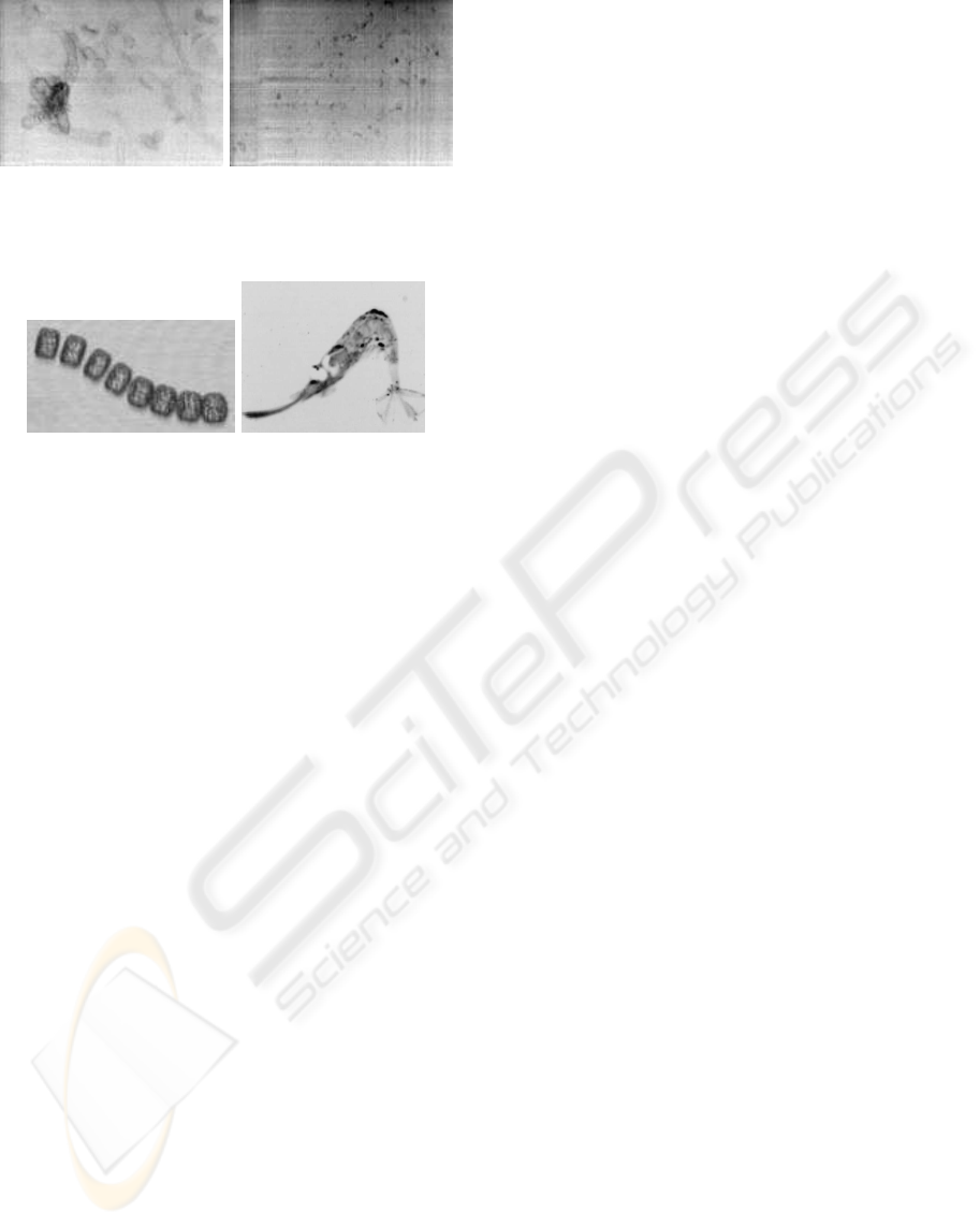
Figure 1: Average images of chain colonial radiolarians

(left) and marine snow from our data set. See Figure 4 for

individual samples. Images throughout this paper are en-

hanced for display by inverting and/or adjusting brightness.

Figure 2: Images from FlowCAM (left) and VPR (right).

sually recognizing marine species from their average

images is extremely difﬁcult, if not impossible.

We applied two very different techniques to au-

tomatically label taxonomic categories of challenging

marine images. The ﬁrst, referred to as the traditional

approach, is common in the machine vision commu-

nity. Processing involves image segmentation, com-

pact feature vector representation, followed by classi-

ﬁcation. Through many years of research, segmenting

an image has remained a non-trivial problem. Solu-

tions are usually not well-deﬁned and most often are

highly dependent on speciﬁc data sets and their appli-

cations. Given the unique characteristics of our plank-

ton images, we propose a novel segmentation tech-

nique that is capable of effectivelyhandling very com-

plex underwater scenes of microscopic organisms.

The second approach, referred to as the biological

approach, is based on (Serre et al., 2005) and is in-

spired by the success of sophisticated visual systems

in primates. With only 2 main computations, correla-

tion mimicking simple cells and maximization mim-

icking complex cells, the model is relatively simple.

Features are constructed from randomly selected im-

age regions. Neither segmentation nor focus of atten-

tion is necessary. Unlike the traditional approach, this

domain independent trait makes the biological system

effectively generalizable. This beneﬁt comes with a

high computational cost, which is far from being real-

time. Investigation of the model complexities led to

modiﬁcations that resulted in a substantial computa-

tional reduction and an improvementin classiﬁcation.

2 RELATED WORKS

2.1 Plankton Classiﬁcation

Two of the most related works are (Blaschko et al.,

2005) and (Lisin, 2006). Blaschko et al. employed a

variety of existing features and classiﬁers. They iden-

tiﬁed plankton in images obtained using a Flow Cy-

tometer And Microscope, FlowCAM (Sieracki et al.,

1998), on which their accuracy was 72.61%. Lisin

studied a kernel density estimation on local bags of

features and proposed a methodology combing multi-

ple global and local features. His algorithm improved

the results obtained by Blaschko et al. on the same

FlowCAM data, achieving 74.84%. He also applied

his technique to images obtained using a VPR (Video

Plankton Recorder), reporting 71.90% accuracy.

Here, we look at a difﬁcult set of video sequences

of several species of tiny underwater organisms (re-

fer to Section 5 for a complete detail). Our images

were obtained using an older VPR that exhibited sig-

niﬁcantly greater noise than the VPR used by Lisin.

There are signiﬁcant differences among the three

marine image sets: FlowCAM, Lisin’s, and our VPR.

Samples of actual images used by Blaschko et al. and

Lisin are shown in Figure 2. Images are mostly well

conditioned. An organism is clearly presented as fore-

ground, though some are partially cropped, and ﬁne

details are apparent. A relatively high contrast sim-

pliﬁes background separation and segmentation.

By comparison, as evidenced in Figure 4, our im-

ages are particularly challenging due to variations

within and between classes, as well as low image

quality and limited resolution. The data exhibit a low

signal-to-noise ratio and signiﬁcant correlated noise.

Detecting and classifying objects are rather difﬁcultin

these images even by humans. Organisms are mostly

localized and typically occupy only small regions.

Many are not captured in their entirety. A number of

organisms are translucent resulting in regions that are

combinations of foreground and background. Some

are distributed, appearing as separate particles, often

in extremely diversiﬁed shapes.

2.2 Biologically Inspired Vision System

Primate effortlessly perceive and efﬁciently use vi-

sual cues to extract reliable information from less than

pristine data. How this fascinating process is exe-

cuted has long been an intriguing question in multiple

disciplines, most notably, neuroscience, physiology,

and psychology. Early pioneers, (Hubel and Wiesel,

1959) discovered simple and complex cells and de-

scribed them as edge detectors. Spatially larger, com-

VISAPP 2010 - International Conference on Computer Vision Theory and Applications

402

Figure 3: Our segmentation applied to two examples of marine images, one on each row, side by side with results of the

technique used by (Lisin, 2006). Shown from left to right are the original image, the intermediate and the ﬁnal results of

Lisin’s approach, and results of our three-step approach, after noise removal, candidate segmentation, and grouping. While

Lisin’s technique fails on these images, our approach successfully segments both organisms from their background.

plex cells are less sensitive to transitional changes.

Later, (De Valois and De Valois, 1988) suggested a

proﬁle of receptive ﬁelds of simple and complex cells,

a structure that resembles Gabor functions.

A model of a biologically feasible vision system

was designed by (Riesenhuber and Poggio, 1999).

They emphasized the two fundamentals: speciﬁcity

and invariance. Their hierarchical model, HMAX,

consisted of linear S layers performing template

matching and nonlinear C layers performing a MAX-

like pooling. They introduced and detailed how the

MAX operation could be a key mechanism for invari-

ance when building complex cells from simple cells.

Serre et al. extended HMAX beyond the cortical

neurons (Serre et al., 2005). On commonly used data

sets, this enhanced system, referred to as the Standard

Model (more detail in Section 4), performed competi-

tively with respect to other state-of-the-art techniques.

3 TRADITIONAL APPROACH

3.1 Image Segmentation

A customized segmentation is developed to overcome

the challenges associated with the data. After signif-

icant exploration of alternative methods, the best re-

sults (Figure 3) are obtained using a 3-step approach:

noise removal, candidate segmentation, and grouping.

Fractional spline wavelet ﬁltering (Blu and Unser,

2003) is employed to clean up noise. A wavelet trans-

form of an image is computed, then thresholded on

the coefﬁcients. A single threshold is empirically de-

termined for all images in the set. Finally, the image is

reconstructed from its thresholded wavelet transform.

A wavelet degree of 3 is used with a threshold of 50.

Noise removal is followed by a segmentation al-

gorithm originally developed to count nuclei in digital

microscopic images (Byun et al., 2006). This candi-

date segmentation consists of 4 steps: median ﬁlter-

ing, thresholding, watershed ﬁltering, and size ﬁlter-

ing. Median ﬁltering with a 5x5 window is performed

to remove more of the remaining noise. Automatic

thresholding attempts to ﬁnd an optimal threshold by

minimizing intra-class variance with respect to parti-

cles and background. The resulting binary image is

processed with watershed ﬁltering and a morpholog-

ical opening operator to remove spurious small parti-

cles, then a size ﬁlter is applied to remove very large

(>5000 pixels) and very small (<5 pixels) particles.

The last step groups all candidate particles within

a certain radius, increasing the particle area and at-

tempting to restore coverage for areas that were re-

moved in previous steps. This improves segmentation

as translucent parts of many organisms are initially re-

moved. However, a sufﬁcient number of widely dis-

tributed parts still remain to indicate the outline of the

particle. A grouping distance of 50 pixels is used,

based on image resolution and expected object size.

3.2 Feature Extraction and

Classiﬁcation

Several types of features are extracted after segmenta-

tion: simple shape descriptors, moments, contour rep-

resentations, texture features, and shape indices. This

set is similar to the set used in (Blaschko et al., 2005).

Simple shapes, computed from each of the seg-

mented particles, include area, perimeter, compact-

ness, ratio of eigenvalues, eccentricity, rectangular-

ity, and convexity. Grayscale moments computed are

mean, variance, skewness, and kurtosis. In addition,

moment invariants as deﬁned by (Hu, 1962) over bi-

nary as well as original grayscale images are used.

A set of texture descriptors is derived from co-

occurrencematrices coveringthe segmented particles.

A co-occurrence matrix is a two-dimensional his-

togram that tracks the number of occurrences of pairs

CLASSIFICATION OF CHALLENGING MARINE IMAGERY

403

of graylevels at each horizontal and vertical displace-

ments. From these matrices, energy, inertia, entropy,

and homogeneity (Haralick, 1979) were calculated as

features. Other texture descriptors were local binary

patterns (Ojala et al., 2002), derived by calculating a

circle of points around a center pixel and assigning

binary weights to the signs of the differences between

these pixels and the center pixel. These patterns are

calculated for each pixel in the segmented particle and

are accumulated into a histogram of counts. Normal-

izing by object size yields the features used.

Shape indices are effective global differential im-

age descriptors for object recognition (Ravela, 2003).

They are functions of the isophote and ﬂowline curva-

tures of the image intensity surface, which are com-

puted using Gaussian derivative ﬁlters. Shape indices

are computed for every pixel in the image, including

background. Histograms of individual shape indices

are calculated and used as features.

Classiﬁcation is done using a Support Vector Ma-

chine (SVM) with a third order polynomial kernel.

The results are based on 10-fold cross validation.

4 BIOLOGICAL APPROACH

The Standard Model (Serre et al., 2005), a framework

for constructing a set of image features, is designed to

be consistent with the structure commonly agreed to

exist in the immediate visual processing of primates.

Primates have a remarkable ability to recognize

an object that has undergone various transformations,

such as afﬁne and perspective projections, or extreme

changes in lighting conditions, and to distinguish sim-

ilar objects belonging to different categories. Un-

derlying this effectiveness is a balance between se-

lectivity and invariance. The Standard Model mim-

ics these mechanisms by interleaving simple S with

complex C layers in a hierarchical feedforward archi-

tecture. Simple cells perform selectivity, responding

strongly only to patterns they are tuned to. Complex

cells are tolerant to changes in scale and translation.

They nonlinearly combine activations and inhibitions

from multiple similarly tuned simple cells.

This structure supports a gradual increase in com-

plexity and invariance of neurons as well as the size of

their receptive ﬁelds along the visual pathway. While

progressing from primitive tokens to deﬁned shapes

and forms, MAX pooling covers larger image regions.

4.1 The Four-layer Standard Model

The ﬁrst layer, S1, resembles simple cells in V1 that

process spatial frequency information. S1 is modeled

by Gabor ﬁlters, extracting edge-like features at 16

scales and 4 orientations. The second layer, C1, simu-

lates complexcells. Neighboring scales and neighbor-

ing pixels of S1 maps are combined using a MAX op-

erator. Subsampling these responses creates C1 maps.

During training, image patches are randomly ex-

tracted from a number of randomly selected C1 maps.

Given an unknown input image, locating an area that

best matches with each of these patches is a process

in S2 and C2. A patch is convolved with C1 maps

of the input, generating S2 maps. Maximizing across

all scales and positions results in a C2 value. Intu-

itively, a feature value indicates how similar a region

in an image is to a particular patch. This procedure

is repeated for every patch, thus constructing for each

input a feature vector of length equal to the number

of training patches extracted. Feature vectors are then

classiﬁed using a supervised one-against-one SVM.

4.2 Modiﬁcation to the Standard Model

One drawback of the Standard Model is its high com-

putational cost precluding real-time operation. Addi-

tionally, with the amount of randomness involved, an

experiment needs to be run repeatedly in order to ob-

tain good statistical estimates. Empirically tracing the

computations, the bottleneck is in correlating training

patches with images. We apply two approaches to re-

duce the number of patches and thus overall compu-

tational cost without sacriﬁcing performance.

Overlaps among Image Patches. Given the size of

an image and a patch, there is a limited number of

patches, n, that can be extracted so no patches overlap,

for example, n is 12 when extracting 32×32 patches

from a 128×96 image. Partial overlaps capture differ-

ent views or different parts of an image and how they

are fused together. Excessive overlaps, on the other

hand, lead to unnecessary duplicates and increase de-

pendency among patches. We prevent an image from

being overly represented with overlapping regions by

extracting a maximum of n patches per image. Instead

of exclusively selecting non-overlapping patches, we

maintain random selection allowing partial overlaps.

Information Contained in an Image Patch. Gen-

erally, a classiﬁer needs to be trained on both fore-

ground and background information. A few back-

ground patches are necessary, but not so many that

they signiﬁcantly increase computations and intro-

duce bias. Our marine data is sensitive to the lat-

ter problem due to uniform underwater background

and organisms occupying only a small area on an im-

age. A large number of extracted regions, especially

smaller ones, are exclusively background.

VISAPP 2010 - International Conference on Computer Vision Theory and Applications

404

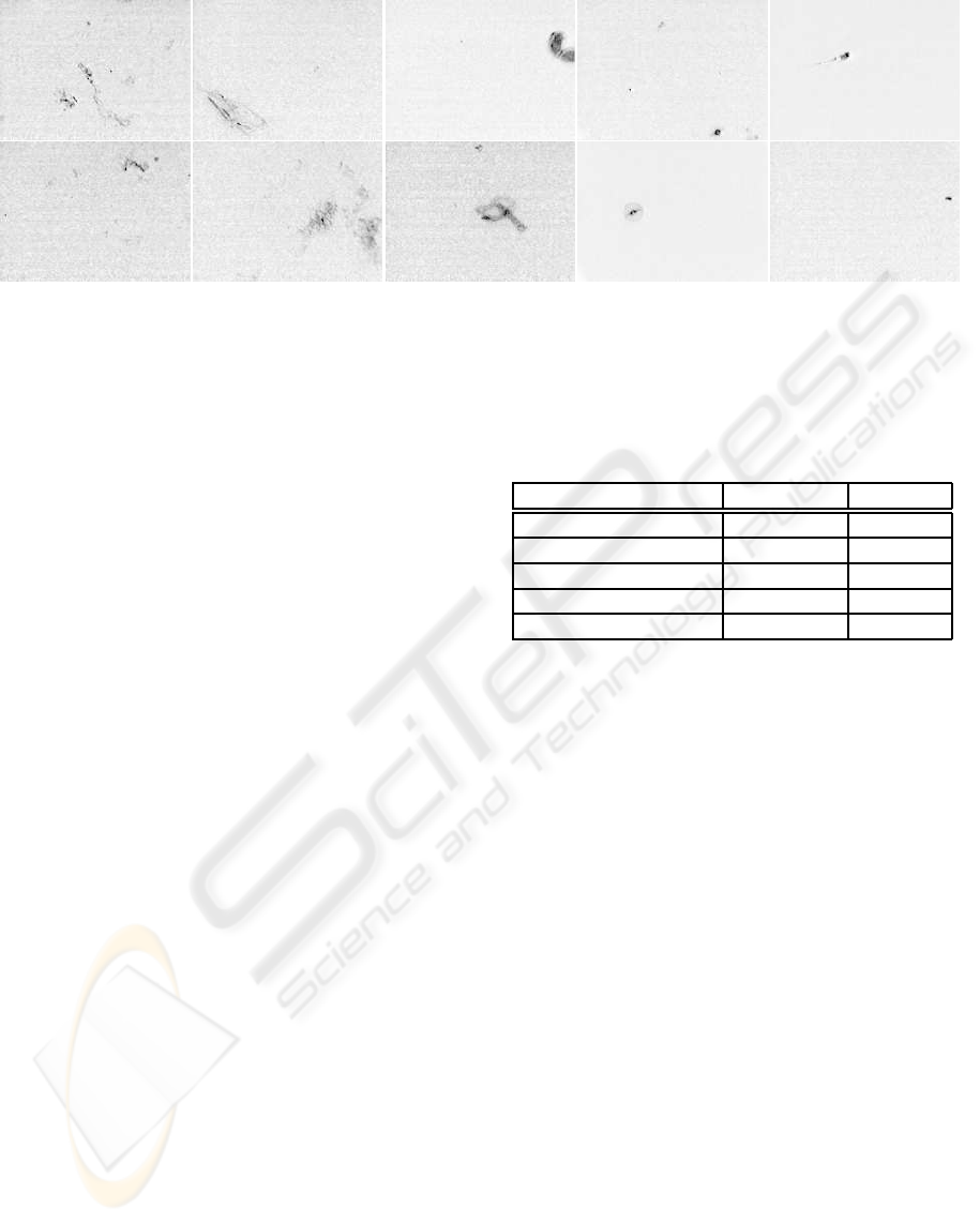
Figure 4: Sample images of our marine data: each column shows two images from each of the ﬁve classes, from left to right,

algal aggregates, Rhizosolenia mats, chain colonial radiolarians, single sphere colonial radiolarians, and marine snow.

We measure information content using entropy.

High entropy signals a heterogeneous ﬁeld, an indica-

tion of activities. These patches likely contain at least

a partial object. A patch with low entropy appears as

a homogeneous ﬁeld, containing no information on

either objects, background, or their border relations.

Therefore, it is safe to exclude low-entropy patches

from a feature set. We eliminate 30% of patches with

the lowest entropy and use the rest as actual templates.

4.3 Implementations

Our Matlab implementation is based on (Serre et al.,

2005), in which preprocessing includes resizing every

image so its height is 140 pixels and its aspect ratio is

preserved. S1 and C1 parameters are left unchanged.

Training patches are extracted from C1 maps at the

second to the ﬁnest scale of Gabor ﬁlters. Patches are

square; 4, 8, 12, and 16 pixels. From a training image,

32 patches are randomly selected, 8 of each size.

A data set is randomly divided into disjoint sets

for training and testing. There are 30 training images

from each class. The rest of the images from a class

with less than 80 images form a test set. Otherwise,

50 test images are chosen. Accuracies are averages

over 25 runs, all of which have different sets of ran-

domly chosen training and testing images. The errors

indicate 95% conﬁdence interval of the mean values.

5 MARINE DATA SETS

The Paciﬁc VPR imagery was collected in the North

Paciﬁc Subtropical Gyre during an August-September

2003 research cruise, which was part of NSF-funded

projects to examine oceanic nitrogen cycling as in-

ﬂuenced by marine diatom and algal aggregate dis-

tribution (Pilskaln et al., 2005). The slowly towed

VPR was lowered 150m from the surface. This un-

Table 1: Classiﬁcation accuracies and running times. Each

runtime is for a single experiment including on-line feature

computations and classiﬁcations, but excluding off-line pre-

processing steps; image segmentation for the traditional ap-

proach and Gabor ﬁltering for the biological approach.

Experiment Speciﬁc Accuracy % Time min

Traditional Approach 76.69 40.83

The Standard Model

no modiﬁcation 78.16±1.11 251.44

patch overlap 79.96±1.16 149.13

overlap and entropy 80.73±1.03 116.88

derwater video microscope system captured images

at 60Hz. An interlaced scan pattern with odd/even

ﬁelds is used. Due to rapid movements of both the

imaging system and objects imaged, raw individual

ﬁelds are interpolated. After post-processing, images

are resized to a resolution of 640×480 pixels.

The data set contains 488 images of marine organ-

isms hand-selected and hand-labeled by oceanogra-

pher experts; examples are shown in Figure 4. Two of

the 5 classes are phytoplankton: algal aggregates and

Rhizosolenia mats. Two are protozoan zooplankton:

chain colonial radiolarians and single sphere colonial

radiolarians. The ﬁfth class is marine snow (organic

detritus). Phyto- and zooplankton are living plant and

animal that drift in the water. Detritus are non-living

particles sinking to the bottom layers of the ocean.

6 RESULTS AND DISCUSSIONS

Classiﬁcation accuracies along with running times of

the experiments are reported in Table 1. Comparing

the traditional approach with the biological model and

its variants, the former has much lower computational

cost, allowing images to be categorized more quickly.

Both approaches accomplish classiﬁcation accuracies

between 76-80%. Given a 75-80% labeling agree-

CLASSIFICATION OF CHALLENGING MARINE IMAGERY

405

ment between expert biologists and 71-75% accura-

cies from similar works by (Blaschko et al., 2005)

and (Lisin, 2006), our techniques perform very well

on this very complex marine data set.

We compare the performance of the Standard

Model with no modiﬁcation versus when the number

of extracted training patches is limited. The latter re-

duces running time by over 40%. Not only is the com-

putational cost signiﬁcantly lower, but also the clas-

siﬁcation results improve (using t-statistic conﬁrms

a signiﬁcant difference at a 95% conﬁdence level).

These results suggest that, without modiﬁcation, over-

lap among patches contains redundant information

and decreases the separability among classes.

Measuring the information content of patches us-

ing entropy effectively removes patches that contain

little to no information relevant to a categorization.

The difference between the two accuracies, both with

overlapping patches constraint applied, but with and

without the use of entropy to select patches, show no

statistical signiﬁcance. The system performs equally

well with 30% less features (without lowest-entropy

training patches), a signiﬁcant saving of a computa-

tional cost. The running time with the entropy selec-

tion process is reduced by over 20% compared to the

system just using constrained patch overlap and by

over 50% compared to the original Standard Model.

7 CONCLUSIONS

The potential of an artiﬁcial vision system based on

biological principles is shown to be quite promising.

A crucial advantage is its independence of image seg-

mentation, a potentially high complexity processing

step. When experimenting with the Standard Model,

we were able to apply it, without re-tuning, and ob-

tain accuracies as good as or better than a traditional

approach, indicating good generalization capability.

To our knowledge, this is the ﬁrst study that ap-

plied a biologically inspired model to a difﬁcult un-

derwater imaging domain. Our experimental results

offer great promise for the analysis of large marine

image data sets collected from unique open-ocean

ecosystems. Automatic identiﬁcation and quantiﬁca-

tion of the plankton and particle components, coupled

with chemical and taxonomic composition analysis,

will facilitate the production of a reﬁned carbon and

nitrogen budgets for this vast region, signiﬁcant to our

understanding of how climate change affects the dy-

namics of ocean ecosystems.

ACKNOWLEDGEMENTS

This work was supported by NSF (OCE-0325167).

REFERENCES

Benﬁeld, M. et al. (2007). RAPID: Research on automated

plankton identiﬁcation oceanography. Oceanography.

Blaschko, M. et al. (2005). Automatic in situ identiﬁcation

of plankton. In Proc. IEEE WACV, pages 79–86.

Blu, T. and Unser, M. (2003). A complete family of scaling

functions: The (α, τ)-fractional splines. In Proc. IEEE

Intl. Conf. Acoustics, Speech, and Signal Processing.

Byun, J. et al. (2006). Automated tool for the detection of

cell nuclei in digital microscopic images: Application

to retinal images. Molecular Vision, 12:949–960.

Culverhouse, P. et al. (2003). Do experts make mistakes?

A comparison of human and machine identiﬁcation of

dinoﬂagellates. Marine Ecology Progress Series, 247.

De Valois, R. L. and De Valois, K. K. (1988). Spatial Vision.

Haralick, R. M. (1979). Statistical and structural approaches

to texture. Proceedings of the IEEE, 67(5):786–804.

Hays, G. C., Richardson, A. J., and Robinson, C. (2005).

Climate change and marine plankton. Trends in Ecol-

ogy and Evolution, 20(6):337–344.

Honjo, S., Manganini, S., Krishﬁeld, R., and Francois, R.

(2008). Particulate organic carbon ﬂuxes to the ocean

interior and factors controlling the biological pump:

A synthesis of global sediment trap programs since

1983. Progress In Oceanography, 76(3).

Hu, M. (1962). Visual pattern recognition by moment in-

variants. IEEE Trans. Information Theory, 8:179–187.

Hubel, D. and Wiesel, T. (1959). Receptive ﬁelds of single

neurons in the cat’s striate cortex. J. of Physiology.

Lisin, D. A. (2006). Image Classiﬁcation with Bags of Local

Features. PhD thesis, Univ. of Mass., Amherst, MA.

Ojala, T., Pietik¨ainen, M., and M¨aenp¨a¨a, T. (2002). Mul-

tiresolution gray-scale and rotation invariant texture

classiﬁcation with local binary patterns. IEEE PAMI.

Pilskaln, C. et al. (2005). High concentrations of marine

snow and diatom algal mats in the north paciﬁc sub-

tropical gyre: Implications for carbon and nitrogen cy-

cles in the oligotrophic ocean. Deep Sea Research.

Ponce, J. et al. (2006). Dataset issues in object recognition.

In Towards Category-Level Object Recognition.

Ravela, S. (2003). On Multi-Scale Differential Features and

their Representations for Image Retrieval and Recog-

nition. PhD thesis, Univ. of Mass., Amherst, MA.

Riesenhuber, M. and Poggio, T. (1999). Hierarchical mod-

els of object recognition in cortex. Nat. Neurosci.

Serre, T., Wolf, L., and Poggio, T. (2005). Object recogni-

tion with features inspired by visual cortex. In Proc.

IEEE CVPR. http://cbcl.mit.edu/software-datasets.

Sieracki, C., Sierackia, M., and Yentsch, C. (1998). An

imaging-in-ﬂow system for automated analysis of ma-

rine microplankton. Marine Ecology Progress Series.

VISAPP 2010 - International Conference on Computer Vision Theory and Applications

406