SEGMENTING COLOR IMAGE OF PLANTS WITH

A SPATIO-COLORIMETRIC APPROACH

Cindy Torres, Alain Clément and Bertrand Vigouroux

Université d’Angers, Laboratoire d’Ingénierie des Systèmes Automatisés (EA 4014)

Institut Universitaire de Technologie, 4 Bd Lavoisier, BP 42018 - 49016 Angers Cedex, France

Keywords: Color, Spatial Organization, Classification, Segmentation, Plants.

Abstract: An unsupervised vectorial segmentation method using both spatial and color information is presented. To

overcome the problem of memory space, this method is based on a multidimensional compact histogram

and an original compact spatial neighborhood probability matrix (SNPM). The multidimensional compact

histogram allows a drastic reduction of memory space without any data loss. Leaning upon the compact

histogram, a SNPM has been computed. It contains all non-negative probabilities of spatial connectivity

between pixel colors. In an unsupervised histogram analysis classification process, two phases are

classically distinguished: (i) a learning process during which histogram modes are identified and (ii) a

second step called the decision step in which a full partition of the colorimetric space is carried out

according the previously defined classes. During the second step of a standard colorimetric approach, a

colorimetric distance like Euclidean or Mahalanobis is used. We insert here a spatio-colorimetric distance

defined as a weighed mixture between a colorimetric distance and the spatial distance calculated from the

SNPM. The vectorial classification method is based on previously presented principles, achieving a

hierarchical analysis of the color histogram by means of a 3D-connected components labeling. Results are

applied to color images of plants to separate plantlets and loam.

1 INTRODUCTION

Segmentation is an important step in the image

processing chain for identifying and partitioning the

different regions of interest in an image. Classically,

the algorithms for segmenting images can be divided

into two families: the ones using the image plane

spatially and the others using the color distribution

of the pixel in the selected color space.

In color images, a pixel is considered as a three-

dimensional (3D) vector whose components depend

on the color space used. When color distribution is

chosen, it is supposed that colors of homogenous

regions give rise to clusters in the color space, each

of them corresponding to a class of pixels. The

different classes are obtained by a cluster analysis or

by means of a color mode detection method

generally based on color histograms. This procedure

assigns each pixel of the image to a class depending

on its color. By connecting pixels from the same

class, regions are constituted.

The entire color information is frequently not

used because of the computation time required. That

is why, most color classification methods are based

on mono or bi-dimensional histograms regardless of

the correlation between color planes is lost. Trémeau

and Laget (Trémeau and Laget, 1995) have

demonstrated however, by the Shannon theory, that

using a multidimensional analysis is more

discriminatory than a mono-dimensional analysis.

To overcome the problem of memory space, Xuan

and Fisher (Xuan and Fisher, 2000) propose to

requantify the color scale by reducing the number of

bits for coding each color component. This

technique is efficient, but it performs an a priori

color classification.

Among segmentation methods using color space

classification, the ones relying on histograms

analysis have the advantage of being unsupervised

but have also the drawback of not taking into

account the spatial information. For the last few

years, a third family of segmentation methods has

appeared: spatio-colorimetric classification methods.

For some images, the loss of the spatial

information conducts to a false segmentation. That

problem was highlighted by Trémeau (Trémeau,

191

Torres C., Cl

ement A. and Vigouroux B. (2010).

SEGMENTING COLOR IMAGE OF PLANTS WITH A SPATIO-COLORIMETRIC APPROACH.

In Proceedings of the International Conference on Computer Vision Theory and Applications, pages 191-196

 SciTePress

1993) and Macaire et al. (Macaire et al., 2006).

With natural color images, the classification

generally leads to an over-segmented image with

small regions scattered through the image. This may

be explained by the lack of correspondence between

some peaks in the color space and significant

regions in the image, or by the merging of too small

peaks with higher ones colorimetrically close but

corresponding to inhomogenous spatial regions. To

cope with these problems, original approaches

taking into account both spatial connectivity and

color information have been proposed by (Macaire

et al., 2006) (Foucher et al., 2001) (Trémeau, 1993)

(Busin et al., 2005) (Noordam and Broek, 2000)

(Comaniciu and Meer, 2002). They have developed

original supervised or not algorithms or fixed

important axioms.

These approaches are facing the double difficulty

of treating a huge quantity of information and

dealing with a high algorithmic complexity.

In this paper we present a new contribution to

unsupervised spatio-colorimetric classification. For

several years, our laboratory has been involved in

developing classification algorithm based on

multidimensional histograms (Clément and

Vigouroux, 2003), (Ouattara and Clément, 2008).

Thanks to the compact histogram (Clément and

Vigouroux, 2001) and an original compact spatial

neighborhood probability matrix, a new

unsupervised vectorial segmentation method taking

into account the full 3D histogram and the spatial

organization of pixels has been developed. This

method is based on a hierarchical analysis of the

histogram. In a standard colorimetric approach,

colorimetic t-uples are attributed to classes

minimizing a colorimetric distance like Euclidean or

Mahalanobis. We insert here a spatio-colorimetric

distance taking into account the information of

pixels neighborhood colors. This distance is defined

as a weighed mixture between a colorimetric

distance and the spatial distance calculated from the

spatial neighborhood probability matrix. The

vectorial classification method is based on the

spatio-colorimetric distance and achieves a

hierarchical analysis of the color histogram using a

3D-connected components labeling.

In a first part, the principle of the compact

histogram is explained and the spatial neighborhood

probability matrix is detailed.

Secondly, the hierarchical unsupervised

classification method is presented and the spatio-

colorimetric distance is defined.

In a third part, the classification method has been

applied to synthetic color images with different

spatio-colorimetric results according the weight

given to spatial and color information. Real images

of plants have been tested, in order to separate

plantlets and loam.

Finally, we discuss previously obtained results,

and propose further development taking into account

the spatial information, during the classification

process, both in the decision and in the learning

steps.

2 COMPACT HISTOGRAM

Segmentation methods based on the analysis of color

histograms are facing the difficulty of treating a

huge quantity of information. For a color image of

resolution NM with each component coded on 8

bits, a standard 3D histogram is an array of 2

cells,

the number in each cell being coded on at least

log

(MN) bits in order to store the greatest number

of pixels. In the case where M=N=256, the standard

3D histogram requires 128 Mo.

A few years ago, we proposed a new way of

coding the nD histograms, leading to the so-called

compact histogram (Clément and Vigouroux, 2001).

Considering that most cells of the standard

histogram are empty, the compact histogram retains

only the C occupied cells. It consists of two arrays

(figure 1): an array of size C×3 to store the colors,

sorted out in lexicographical order, and an array of

size C×1 for the corresponding populations of

pixels. Since C is lower than MN, the compact

histogram occupies less memory space, although it

contains the full color information present in the

image. For a 256256 image with color components

coded on 8 bits, the memory space required is less

than 500 ko.

population

...

255

251

254

Figure 1: Example of 3D compact histogram for a RGB

color image (8 bits per component).

3 SNPM

Taking into account previous researches in spatio-

colorimetric classification such as (Trémeau, 1993)

and (Macaire et al., 2006), it is interesting to have a

VISAPP 2010 - International Conference on Computer Vision Theory and Applications

192

structure like a co-occurrence matrix, containing

color pixels neighbors information.

For a given spatial direction, a co-occurrence

matrix calculates how often a pixel with a color c

occurs adjacently to a pixel with a color c. Other

spatial relationships between pixels may be

specified. That kind of structure is generally used to

analyze grey levels textures. Without any

requantization, a memory space of 256

cells is

occupied.

A color image presents a maximum of 256

colors, its corresponding standard co-occurrence

matrix will have 256

cells. Let C be the number of

different colors in an image, C is usually lower than

256

. Nevertheless, a co-occurrence matrix with C

cells requires a huge memory space. That is why a

Spatial Neighborhood Probability Matrix (SNPM),

requiring a reduced memory space, has been

proposed.

This matrix specifies the probability to find a

pixel with the color c in the neighborhood of a

pixel with the color c, knowing that we have this

pixel with the color c.

Given a color pixel p

c

, the neighborhood v

c

)

is the set of all pixels whose distance from p

c

equal to d. For d=1, this neighborhood is defined by

a 4 or 8 connexity. For d>1, a form (disk, square,

diamond…) defines the connexity. The full

neighborhood V(p

c

) is then defined as :



V ( p



)  v

i1

( p



)

(1)

Let h

c

) be the compact histogram associated

with v

c

). A weighed histogram H(p

c

)

corresponding to V(p

c

) is defined as:



H( p



)  h

i1

( p



)  (1 d  i)

(2)

where  is a weighing operator which multiplies

each compact histogram h

populations. Thus in

V(p

c

), colors weights are higher when colors

correspond to pixels close to p

c

. If {c} is the set of

all pixels having the color c, H

c

is defined as:





 H(p



j1

Card({ c



})

)

(3)

The SNPM is a cell array of size Cx1, with C the

number of different colors in the image. Each cell i,

1≤ i ≤C, contains the corresponding H

ci

whose

population has been normalized to 1 in order to

express probabilities. The probability P(c  H

c

)

to find a pixel with the color c in the neighborhood

of a pixel with the color c in the image, is directly

given by the c entry of the histogram associated

with the c cell in the SNPM. By construction,

SNPM contains C compact histograms, each

histogram having less than C cells. Memory space

required by SNPM is lower than the one required by

a co-occurrence matrix, even coded in a compact

form with C

cells.

The spatial distance ds(c, c) is defined from

SNPM as the minimum between [1-P(c  H

c

)]

and [1-P(c  H

c

)].

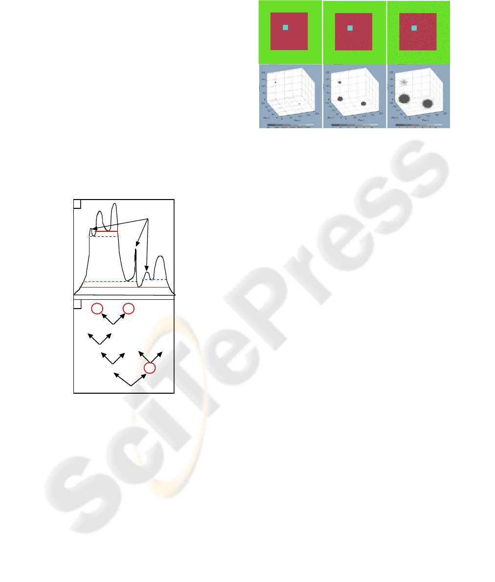
4 HIERARCHICAL

CLASSIFICATION

The classification process through an unsupervised

analysis of color histograms is an original 3D

extension of the 2D limited method proposed in

(Clément and Vigouroux, 2003). Colors

classification is carried out in two steps: the learning

step and the decision step.

The learning step is a hierarchical decomposition

of populations in the 3D histogram. For each level of

population p

, peaks P

are identified by a connected

components labelling process: first, the color

compact histogram is thresholded for populations

greater than or equal to p

and a binary 3D matrix is

reconstructed in the same way as a standard

histogram but with only one bit per cell. Secondly,

the binary matrix is labelled in 3D connected

components. Each peak identified by a connected

component is then iteratively decomposed into

narrower peaks, beginning from population 0.

Thanks to (Ouattara and Clément, 2008), the

algorithm considers only existing populations in the

compact histogram, jumping from one to the next in

ascending order. A peak is then labelled as

significant if it represents a population greater than

or equal to a threshold S (expressed in percent of the

total population in the histogram). The procedure is

illustrated in figure 2 (drawn in one dimension for

clarity). We shall name kernels K

the peaks

corresponding to circled leaves in part b of figure 2.

In other words, kernels are significant peaks (part of

figure 2) without descendants in the hierarchical

decomposition tree (e.g., figure 2 shows five

significant peaks P

(i = 0 to 4) and three kernels K

(i = 2, 3, 4)). The number of classes N

is taken

equal to the number of kernels (the class

corresponding to kernel K

is noted C

). Therefore N

depends on the threshold S, i.e. on the precision the

image colors are analyzed with.

SEGMENTING COLOR IMAGE OF PLANTS WITH A SPATIO-COLORIMETRIC APPROACH

193

In the decision step, the mass center µ(K

) of

each kernel K

is calculated in the color space. Let us

denote by c the color corresponding to the point of

coordinates (r,g,b) in the color space. Two cases

appear: if (r,g,b) belongs to K

, color c is attributed

to class C

; if not, let us denote by P

the peak

(r,g,b) it belongs to; color c is attributed to class C

corresponding to kernel K

, son of P

, such that

d[µ(K

), (r,g,b)] is minimum, where d[c, c] is a

spatio-colorimetric distance between c and c.

The spatio-colorimetric distance (dSC) is

expressed by equation (4):

dSC(c, c) =  ds(c, c) + (1-) dc(c, c) (4)

where dc(c, c) is a colorimetric distance between

c and c like Euclidean or Mahalanobis and

ds(c,c) the spatial distance as defined from the

Compact SNPM. , 0≤  ≤1, gives more or less

weight to the spatial or colorimetric information.

(

)

(

)

(

)

peak population < S

Figure 2: An example of hierarchical decomposition. The

circled leaves (part b) correspond to significant peaks as

obtained at the end of the iterative decomposition (solid

lines in part a), whereas leaves marked < S (part b)

correspond to insignificant peaks (dotted lines in part a).

5 RESULTS

A synthetic RGB color image with 256x256 pixels,

coded on 24 bits (8 bits per component) each, is used

as a probe image to test the algorithm. This image is

composed of three regions with pure colors: 2

regions with an important population the red and the

green ones, and another composed of few pixels, the

blue one. As shown in the RGB histogram (figure

3,a2), the blue region is colorimetrically closer to the

green region than the red one.

(a1,a2) (b1,b2) (c1,c2)

Figure 3: This figure is composed of three images: a1, b1

and c1, and their corresponding histogram a2, b2 and c2.

Image a1 is the original probe color RGB image (8 bits per

component). Images b1 and c1 are corrupted probe

images; b1 is named lowNoise and c1 highNoise. In

histogram a2, the points have been enlarged for a better

visibility.

RGB-histogram (a2) reveals the presence of

three classes. In order to evaluate the interest of the

classification algorithm, the colorimetric

components of the probe image have been corrupted

by an additional uncorrelated Gaussian noise: being

, N

three matrices of marginal centered

noise with the same standard deviation  = 0.02 for

the image lowNoise (figure3 b1) and  = 0.05 for

the image highNoise (figure3 c1). The alteration of

the probe image constituted of the three colorimetric

planes P

, P

is given by P

(i  {r,g,b}).

Considering that the blue region’s population is

insignificant, threshold S (defined in the

Hierarchical classification part) has been adjusted

consequently.

Firstly, the classification algorithm has been run

with  = 0 (defined in the Hierarchical classification

part) to neglect the spatial information. The

segmentation obtained is the same for the three

images, and is presented in figure 4(a). Two classes

have been identified, one corresponding to the green

region, another corresponding to the red region.

Insignificant blue values have been classified with

the green region that is colorimetrically the closest.

Secondly,  has been adjusted to take into

account the spatial information ( > 0). The

neighborhood distance d (defined in the Compact

spatial neighborhood probability matrix part) has

been chosen to cover the blue region while

remaining inside the red region. Results are

presented in figure 4(b).

VISAPP 2010 - International Conference on Computer Vision Theory and Applications

194

(a) (b)

Figure 4: (a) is the classification result of figure 3 (a1, b1

and c1) when  = 0.

(b) is the classification result of figure 3 (a1, b1 and c1)

when  > 0, and with a value of neighborhood distance d

covering the blue region.

The segmentation obtained is the same for the

three images. Two classes have been obtained, one

corresponding to the green region only, and the other

one merging the blue and the red regions. Spatially,

blue pixels are closer to red ones and so dSC (blue,

red) is lower than dSC (blue, green).

6 APPLICATION TO PLANTS

IMAGES

This classification method has been used to segment

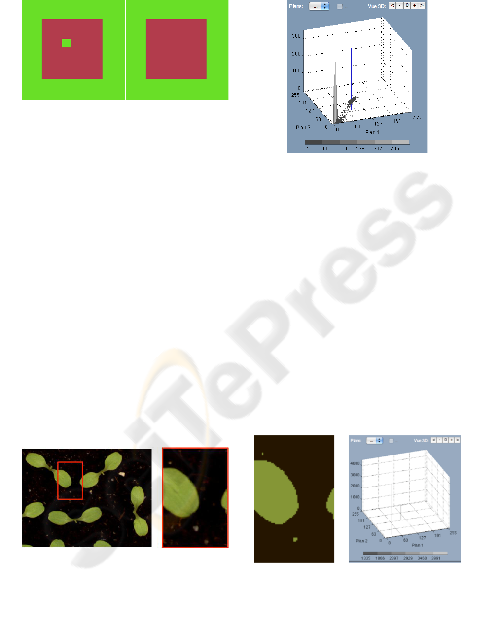
plants images. Figure 5(a) is a RGB image of 7-day

lettuce plantlets, each pixel coded on 24 bits (8 bits

per component). It has been photographied with a

tri-CCD camera, and lettuces were highlighted with

a halogen lamp. The lettuce seeds are sowed on

loam. The loam is heterogeneous, that is one of the

difficulties to segment these images. With color

classification, some regions in the loam are

recognized as plants instead of loam. Figure 5(b) is a

zoom of figure 5(a).

(a) (b)

Figure 5: 7-day lettuce plantlets RGB image (a), with a

zoom (b).

Figure 6: Histogram (presented with the first two

dimensions only for a better visibility) of figure 5(b).

Color points corresponding to the small noisy regions

scattered in the loam, have been highlighted and pointed in

blue.

Figure 6 is the histogram (presented with the first

two dimensions only for better visibility) of the

image, the color points corresponding to the small

noisy regions scattered in the loam, have been

highlighted and pointed in blue. In the following,

these colors will be called color noise.

Firstly, the classification algorithm has been run

with  = 0 to neglect the spatial information and

obtain a color segmentation. Threshold S has been

adjusted in order to ignore the small regions

scattered in the loam. The result is presented in

figure 7(a), with its corresponding 2D histogram in

figure 7(b). The color points (color noise)

corresponding to these insignificant regions were

colorimetrically closer to the green region (color of

the leaf) than the black region (loam). During the

second step of the classification, these colors have

been merged with the green class.

(a) (b)

Figure 7: (a) Color segmentation of image 6(b) with  = 0.

(b) Histogram (presented with the first two dimensions

only for better visibility) of figure 7(a).

SEGMENTING COLOR IMAGE OF PLANTS WITH A SPATIO-COLORIMETRIC APPROACH

195

On another hand,  has been adjusted to take into

account the spatial information ( > 0). The

neighborhood distance d (defined in the Compact

spatial neighborhood probability matrix part) has

been chosen to cover the small regions. Results are

presented in figure 8. Colors of the small regions

have been merged with the black class (loam)

because spatially, noisy pixels are closer to black

ones and so dSC (color noise, black) is lower than

dSC (color noise, green).

Figure 8: Spatio-colorimetric segmentation of figure 5(b).

7 DISCUSSION AND

PERSPECTIVES

Encouraging results have been obtained with the

proposed unsupervised vectorial hierarchical spatio-

colorimetric classification. However, the method

relies on two new parameters:  and the

neighborhood distance d, which are difficult to fix

without an a priori knowledge of the image to be

segmented. The results obtained have shown

efficiency for a neighborhood covering small

regions, with insignificant population. These regions

cannot correspond to classes during the learning step

regarding threshold S. They are merged during the

second step, where the spatial information has been

introduced. The weight of the spatial information

depends on , which is correlated to the colorimetric

distance between these small regions and the others,

that is why both  and distance d are difficult to

evaluate a priori.

Wider colorimetric regions could be treated

introducing the spatial information during the

learning step of the classification. Actually, if a

color population is high enough, it will be a kernel in

the histogram and will form a class. If this class does

not correspond to a spatial region, the problem

cannot be solved increasing the neighborhood

distance d. On the other hand, the hierarchical

decomposition of the histogram could be constrained

to form classes which satisfy a spatio-colorimetric

homogeneity criterion.

REFERENCES

Busin L., Vandenbroucke N., Macaire L., Postaire J.G.,

2005. Colour space selection for unsupervised colour

image segmentation by analysis of connectedness

properties. International Journal of Robotics and

Automation, 20(2):70-77.

Clément A., Vigouroux B., 2001. Un histogramme

compact pour l’analyse d’images multi-composantes.

Actes du 18ème colloque sur le traitement du signal et

des images GRETSI' 01, Toulouse, France, vol. 1, p.

305-307.

Clément A., Vigouroux B., 2003. Unsupervised

segmentation of scenes containing vegetation

(Forsythia) and soil by hierarchical analysis of bi-

dimensional histogram. Pattern Recognition Letters,

nº24, p. 1951-1957.

Comaniciu D., Meer P., 2002. Mean Shift: A Robust

Approach toward Feature Space Analysis. IEEE

Trans. Pattern Analysis Machine Intell., 24(5):603-

619.

Foucher P., Revollon P., Vigouroux B., 2001.

Segmentation d'images en couleurs par réseau de

neurones : application au domaine vegetal. Actes du

congrès francophone par vision par ordinateur

(ORASIS), Cahors, France, 309-317.

Macaire L., Vandenbroucke N., Postaire J.G., 2006. Color

image segmentation by analysis of subset

connectedness and color homogeneity properties.

Computer Vision and Image Understanding, Elsevier,

102:105–116.

Noordam J., Broek W.V.D., 2000. Geometrically guided

fuzzy c-means clustering for multivariate image

segmentation. International Conference on Pattern

Recognition, 1:462–465.

Ouattara S., Clément A., 2008. Unsupervised Image

Segmentation by Multi-Dimensional Compact

Histograms Analysis. ClasSpec’08, October 15th

2008, Lens, France.

Trémeau A., Laget B., 1995. Quantification de la couleur

et analyse d'image, Traitement du signal.

Trémeau A., 1993. Contribution des modèles de la

perception visuelle à l'analyse d'image couleur, PhD

thesis, University of Saint-Etienne, France.

Xuan G., Fisher P., 2000. Maximum likelihood clustering

method based on color features. Proceedings of the

First International Conference on Color in Graphics

and Image Processing, Saint-Etienne, France, p. 191-

194.

VISAPP 2010 - International Conference on Computer Vision Theory and Applications

196