SHAPE AND SIZE FROM THE MIST

A Deformable Model for Particle Characterization

Anders Dahl

†

, Thomas Martini Jørgensen

‡

, Phanindra Gundu

‡

and Rasmus Larsen

†

Technical University of Denmark, DTU Informatics Lyngby

†

, DTU Photonics Ris

‡

, Denmark

Keywords:

Particle analysis, Deconvolution, Depth estimation, Microscopic imaging.

Abstract:

Process optimization often depends on the correct estimation of particle size, their shape and their concen-

tration. In case of the backlight microscopic system, which we investigate here, particle images suffer from

out-of-focus blur. This gives a bias towards overestimating the particle size when particles are behind or in

front of the focus plane. In most applications only in-focus particles get analyzed, but this weakens the statisti-

cal basis and requires either particle sampling over longer time or results in uncertain predictions. We propose

a new method for estimating the size and the shape of the particles, which includes out-of-focus particles. We

employ particle simulations for training an inference model predicting the true size of particles from image

observations. This also provides depth information, which can be used in concentration predictions. Our

model shows promising results on real data with ground truth depth, shape and size information. The outcome

of our approach is a reliable particle analysis obtained from shorter sampling time.

1 INTRODUCTION

Visual inspection of particles is often essential for op-

timizing industrial processes. Examples can be parti-

cles in a dissolution, as for instance in a fermentation

process, or particles in gas, such as the coal particles

from a power plant. A vision-based system can pro-

vide knowledge about particle distribution, size and

shape, and these parameters are important for process

control. The choice of the analysis method and the

image quality affects the process control, and as a re-

sult both the analysis and image acquisition should be

chosen carefully.

The motivation of our work is an industrial endo-

scopic inspection system equipped with a probe that

can be placed inside the process

. Images are ac-

quired from the tip of the probe, which also contains

a light source placed in front of the camera. The

resulting camera setup depicts particles as shadows,

see Figure 1. Visual appearance of the particles de-

pends on the optical properties of the camera setup,

the distance of the particles to the focus plane, and the

physical reﬂectance properties of the particles. The

depth of ﬁeld of the camera optics is narrow and the

particles get blurred as they move away from the fo-

cus plane, which introduces uncertainty of the particle

PROVAEN – Process Visualisation and Analysis EN-

doscope System (EU, 6

Framework)

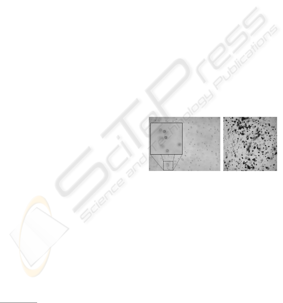
(a) (b)

Figure 1: Examples of particle images. (a) spherical trans-

parent particles all 25 µm in diameter, and (b) a typical im-

age to be analyzed depicting spray particles.

characterization, see Figure 2. Employing a strategy

where only in-focus particles are analyzed can be a

good solution, but in situations with few particles or

short inspection time this approach will give an un-

certain estimate due to low sample size. As a conse-

quence it can be necessary to perform the analysis of

the blurred particles as well.

Deblurring. In a linear system the image formation

can be described as the linear convolution of the ob-

ject distribution and the point spread function (PSF).

Hence, to reduce the blur from out of focus light, ide-

ally the mathematical process of deconvolution can

be applied. However, noise can easily be enhanced if

one just implements a direct inverse operation, so the

Dahl A., Martini Jørgensen T., Gundu P. and Larsen R. (2010).

SHAPE AND SIZE FROM THE MIST - A Deformable Model for Particle Characterization.

In Proceedings of the International Conference on Computer Vision Theory and Applications, pages 36-43

DOI: 10.5220/0002830500360043

 SciTePress

Figure 2: Illustration of the particles relative to the focus

plane. (a) particles in the 3D volume (b) can potentially

appear as a function of the distance to the focus plane.

inverse has to be regularized. Different regularizers

can be employed, for example iteratively deconvolv-

ing the image (Lucy, 1974), (Richardson, 1972), or

using a Wiener ﬁlter (Wiener, 1964). Alternatively,

a maximum entropy solution can be chosen, which

aims at being mostly consistent with data (Narayan

and Nityananda, 1986), (Starck et al., 2002). These

methods assume a known PSF. When this is not the

case, blind deconvolution can in some cases be ap-

plied recovering both the PSF and the deconvolved

image. Typically this is solved by an optimization

criterion based on known physical properties of the

depicted object (Kundur and Hatzinakos, 1996).

These methods are based on the assumption of

a known – possibly space-dependent – PSF for the

whole image. For many optical systems it is difﬁcult

to calculate a theoretical PSF with sufﬁciently accu-

racy to be used for deconvolution. Also it can be quite

difﬁcult to measure it experimentally with sufﬁcient

resolution and accuracy. In our case the particles of

concern are illuminated from the back and in this re-

spect it resembles the case of bright light microscopy.

Such an imaging system is not exactly a linear de-

vice but in practice it is almost so. However, in the

bright ﬁeld setting the ”simple” PSF is compounded

by absorptive, refractive and dispersal effects, making

it rather difﬁcult to measure and calculate it.

Methods for local image deblurring, which is

needed for our problem, include iteratively estimat-

ing the blur kernel and updating the image accord-

ingly in a Bayesian framework (Shan et al., 2008).

Another approach is to segment the image and esti-

mate an individual blur kernel for the segments (Cho

et al., 2007; Levin, 2007). Blur also contains infor-

mation about the depicted objects. This has been used

by (Dai and Wu, 2008; Shan et al., 2007), where they

obtain motion information by modeling blur. With

a successful deblurring, e.g. based on one of these

methods, we will still have to identify the individual

particles. Instead, we suggest here to build a particle

model.

Particle Modeling. Most particles have a fairly

simple structure, typically being convex and close to

circular or elliptical. This observation can be used for

designing a particle model. In (Fisker et al., 2000)

a particle model is build for nanoparticles based on

images obtained from an electron microscope. An el-

liptical model is aligned with the particles by maxi-

mizing the contrast between the average intensity of

the particle and a surrounding narrow band. Particles

in these images are naturally in focus.

Ghaemi et al.(Ghaemi et al., 2008) analyze spray

particles using a simple elliptical model. However,

only in-focus particles are analyzed, and out of focus

particles are pointed out as a cause of error. In addi-

tion, they mention the discretization on the CCD chip

to be problematic, and argue that particles should be

at least 40-60 pixels across to enable a good shape

characterization.

Under the assumption that images are smooth and

by modeling the out of focus blur, we are able to ex-

perimentally show that we can obtain reliable shape

and size information from particles smaller than 40-

60 pixels in diameter. The main contribution of this

paper and the basis for our experiments is a parti-

cle model, which is used for characterizing particle

shape, size and blur. In Section 2 we describe our par-

ticle model and how it can be used for particle char-

acterization. We experimentally validate the particle

model in Section 3. Lastly, in Section 4 we discuss the

obtained results, and we conclude the work in Section

2 METHOD

The goal of the proposed method is to obtain informa-

tion about the true size and shape of an out of focus

particle. Our idea is to learn particle appearance from

observations of particles with known position relative

to the focus plane. By comparing the appearance of

an unknown particle to the training set, we can predict

how the particle would appear, if it was in focus. As

a result we obtain information about the true particle

size and shape.

To facilitate this, the particles must be character-

ized in a way that describes the appearance as a func-

tion of blur well. Furthermore, particles should be

easy to compare. We will now give a short description

of how particles are depicted, and then explain the de-

tails of our particle model and descriptor. Finally we

describe the statistical model for depth estimation.

Experimental Setup. The particle analysis is based

on backlight where the particles appear as shadows.

Real image examples are shown in Figure 1 and Fig-

ure 2 illustrates the experimental setup. Notice that

all particles in Figure 1(a) are the same size of 25µm,

SHAPE AND SIZE FROM THE MIST - A Deformable Model for Particle Characterization

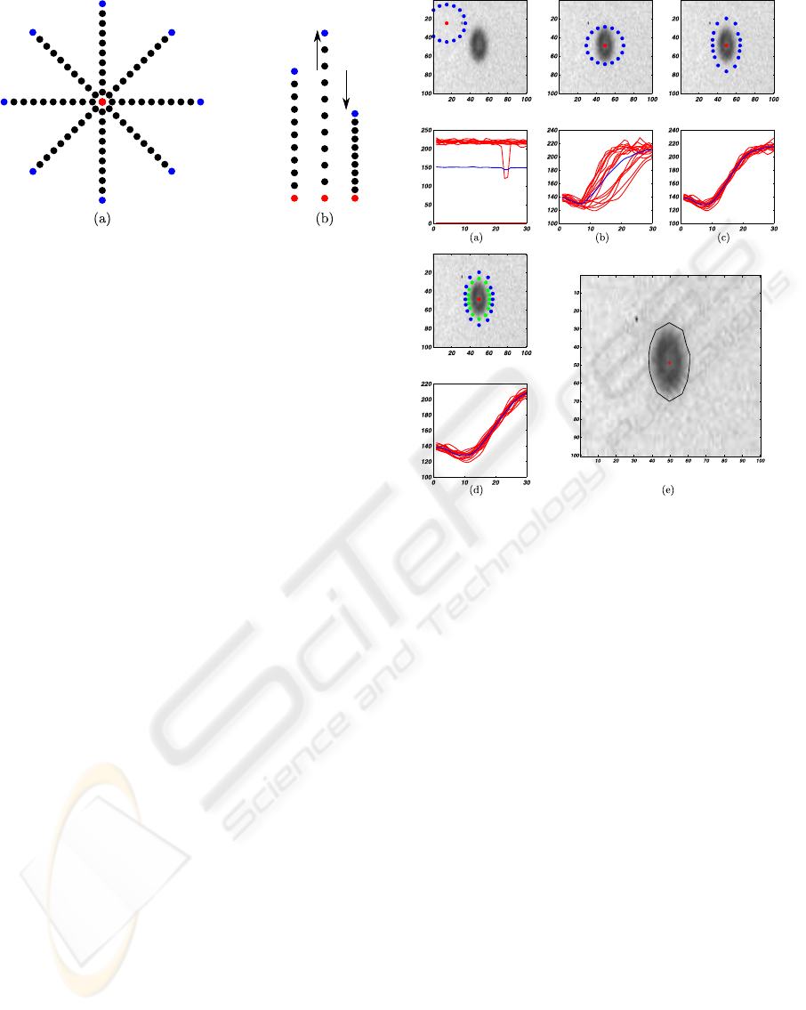
Figure 3: Intensity sampling with the particle model. Radial

sampling pattern of our model with 10 sampling steps from

the center point, marked with red, to the end of the radial

line marked with blue. There are 8 radial sampling lines in

this example (a). Each radial sampling line can be deformed

by stretching or compressing the line while keeping equal

distance between the sampling points (b). This stretch of

the individual sampling lines is what deforms our model.

but the blur makes them appear very different. Out of

focus blur occurs both in front and behind the focus

plane, but it is hard to tell if an observed particle is in

front or behind, because the blur looks the same. As

a consequence we have chosen to model the particles

as a function of absolute distance to the focus plan,

which is shown in Figure 2. In Section 3 we experi-

mentally show that these are reasonable assumptions.

Particle Analysis Model. The objective is to design

a model that encodes information about the particle’s

size, shape and blur. Our model is based on the obser-

vation that particles show close to radial symmetry. If

we sample along line segments from the center of the

particle, we expect to see the same intensity pattern or

a scaled version of this pattern. This is the idea that

we base our particle model on, which is illustrated in

Figure 3.

Our particle prediction is based on the following

Y = [s

, r

, d

]

= f (c

, r

, I

), (1)

where (c

, r

, I

) are the observed spatial position,

shape and image appearance respectively, f is the

function mapping observations to the vector Y con-

taining the model prediction (s

, r

, d

), which is the

true size, shape and distance to the focus plane. We

will now give the details of the particle model and

then explain how the parameters of this model are

used for predicting the particle characteristics.

We sample n radial lines form the center coor-

dinates c

placed with equal angle around the cen-

ter point. A particle descriptor is obtained by sam-

pling the image intensity along these radial lines at m

equidistant positions relative to the lengths of the ra-

Figure 4: Particle alignment and deformation. The image

shows the particle, the red dot is the center, and the blue

dots are the radial endpoints. The red curves show the in-

tensity pattern along the individual radial lines and the blue

is the average. The blob is initialized in (a), translated in

(b), deformed in (c), the size is found in marked with green

points (d) resulting in the segment in (e). Note that despite

a very poor initial alignment the model ﬁnds the object very

precisely. Also note how uniform the intensity pattern be-

comes by deformation.

dial lines. This intensity descriptor is denoted I

. The

length of the radial lines are stored in the r

vector,

which characterizes the particle shape.

Alignment with Image Data. Adapting the model

to the image observations is done in two steps. First

by changing the center position, which translates the

model, and secondly by changing the length of the

radial lines, which deforms the shape of the model.

Both operations will change the intensity descriptor,

which is utilized for ﬁnding an optimal particle char-

acterization. As a preprocessing step for noise re-

moval we convolve the image with a Gaussian kernel

with standard deviation σ.

The particle model has to be initialized by a rough

estimate of the particle size and position, e.g. us-

ing scale space blob detection, see (Lindeberg, 1994).

To obtain the center position of a particle we use an

optimization criterion based on radial symmetry and

VISAPP 2010 - International Conference on Computer Vision Theory and Applications

intensity variance. The reasoning for the ﬁrst crite-

rion is that particles are typically radially symmetric.

Based on that we initiate our particle model with ra-

dial lines of equal length. We expect the radial lines

to have highest similarity when they are sampled from

the particle center, also for particles that are not spher-

ically shaped. The variation criterion is based on the

fact that the intensity descriptor has high variation

when sampled on a particle and low otherwise. This

turns out to be very important for the robustness of

the alignment. The minimization problem becomes

argmin





∑

i=1

||I

−

I||



− ξσ



, (2)

where

I is the mean intensity descriptor, and the

sum of normed descriptor differences is weighed by

η. σ

is the standard deviation of the mean descriptor,

which is weighed by ξ. This alignment is optimized

by simple gradient decent, by moving in the steep-

est decent direction until an optimum is reached. The

procedure is repeated with ﬁner step size, until a de-

sired precision is obtained.

After an optimal particle position has been found,

the particle shape is optimized to the image data by

changing the length of the radial sampling lines

argmin



∑

i=1

||I

−

I||



, (3)

hereby minimizing the difference between the av-

erage descriptor and the individual radial descriptors.

This optimization is done similarly to the positioning,

also using gradient decent and reﬁning the step size

when a minimum is reached. The length of the ﬁnal

radial lines are normalized to sum to the same as orig-

inal radial lines lengths.

The particle model results in an observed charac-

terization as follows

x = {c

, r

, I

}, (4)

containing the center position denoted c

which

is a 2D vector, the length of the radial line segments

denoted r

which is a n-dimensional vector, and the

intensity pattern I

which is m-dimensional. It is esti-

mated as the mean I

∑

i=1

, where I

is the radial

pattern of line segment i. It should be noted that the

difference between the line patterns have been mini-

mized, so we model the remaining difference as noise,

and as a result the averaging will smooth this noise

and make the estimate robust.

Modeling the particle will create an independent

characterization of the size, shape and blur, which is

illustrated in Figure 3. Particle shape is encoded in

the length of the radial line segments, and the particle

size can be obtained from a combination of the radial

intensity pattern and the length of the line segments.

The intensity pattern I

has a shape that bends off to

become indistinguishable from the background, see

Figure 4, and the particle boundary is estimated at this

point. We found a function of the total variation to be

good way of estimating this. We estimate the total

variation as the sum of absolute differences of I

and

we obtain the distance as

= argmax

∑

m− j

i=1

||I

− I

i+1

|| − c

∑

m−1

i=1

||I

− I

i+1

j ∈ {1, ..., m − 1}, (5)

which is the normed total variation. The constant

c inﬂuences the estimated size of the particle.

Statistical Analysis. The blur is encoded in the ra-

dial pattern descriptor (I

), which we use as input for

estimating the distance to the focus plane. We use a

linear ridge regression to obtain the depth. The model

is d

= I

, where β

is the coefﬁcients of the regres-

sion model. We obtain the model parameters from a

training set with known distance to the focus plane by

solving β

= (I

+ λI)

−1

∗

, where d

∗

is the dis-

tance of the training data. See for example (Hastie

et al., 2005) for a detailed description of ridge regres-

sion.

Table 1: Model parameters.

Parameter Value

Radial lines (n) 8

Sampling steps (m) 40

Sampling distance (pixels) 30

Length constant (c) 0.35

Gaussian blur - simulated (σ) 5

Gaussian blur - real (σ) 1

Radial similarty (η - Equation 2) 1

Variance weight (ξ - Equation 2) 4000

3 EXPERIMENTS

In this section we will experimentally show the per-

formance of our particle model. We want to investi-

gate the precision and accuracy of our model. By pre-

cision we mean how good our model is in predicting

the true size, shape and particle depth. The accuracy

refers to variation in the model predictions. The ex-

periments are conducted in relation to size estimation,

shape estimation and the particles distance to the fo-

cus plane. For these experiments we chose the param-

eter shown in Table 1. Furthermore, we investigate

SHAPE AND SIZE FROM THE MIST - A Deformable Model for Particle Characterization

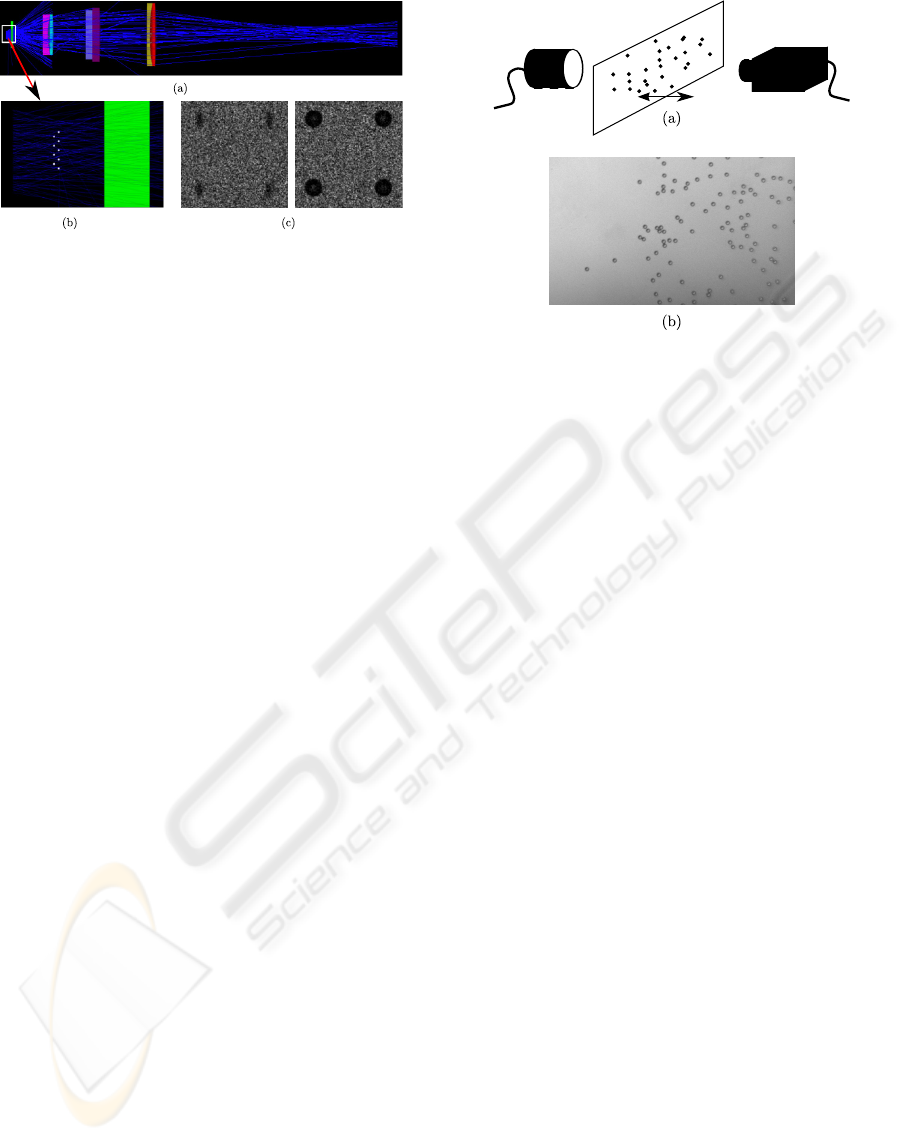
Figure 5: Optical simulation in Zemax. (a) back illumina-

tion with a diffuse light source of 2 mm

with wavelengths

of 480-650 nm with transparent particles. (b) zoom on the

particles and (c) examples of 50 µm out of focus ellipsoid

particels (50 µm × 16.7 µm) and spherical in focus particles

(50 µm).

the robustness of the input parameter choices, which

concerns number of radial lines, number of sampling

steps, sampling distance, optimization weights, see

Equation 2, and the initial position and size estimates

of the particles.

Data. The endoscopic probe consists of three dou-

blets with different powers separated as shown in Fig-

ure 5. The distance between the object plane (parti-

cles) and the ﬁrst optical element, which is a cover

plate, is just 1 mm. The separations between the op-

tical elements up to the CCD is so maintained and

optimized to provide a magniﬁcation of 6. The de-

sign is performed in Zemax optical design software.

The total track length from object to image (particles

to CCD) is 25 cm and the optical resolution of the

system is 2 microns. The entire visible wavelength

region is used to optimize this system (480-650 nm).

The depth of focus at the object side is computed to

be +/- 75 microns when deﬁned by a drop of more

than 90% of the modulation transfer function. To in-

corporate the real situation of illumination with back

light of spherical and ellipsoidal particles, modeling is

done in a non-sequential mode in Zemax, which can

handle diffuse light and 3D particles. The diffuse light

source is located a few millimeters behind the parti-

cles and emits light in the speciﬁed wavelength range

randomly over a 15 degrees angle. The particles used

are transparent with refractive index of 1.6 at 555 nm

wavelength. Several million rays per simulation were

used to generate a single image with particles. Imag-

ing is done using a CCD array with 4 Megapixels of

7 micron pitch.

The real data set consists of particles in water sus-

pension placed between two glass sheets, which have

been moved with µm precision relative to the focus

plane. 25 µm particles are shown in Figure 6.

Figure 6: Setup for acquiring real data. (a) particles placed

between glass sheets that can be moved relative to the cam-

era. (b) image example with LED back illumination and 25

µm spherical transparent particles.

Size Experiment. In this experiment we investigate

the robustness of our size estimation. We have both

tested the mean value and standard deviation of the

estimated size, and how it depends on the distance

to the focus plane. The results are shown in Figure

7. The ﬁrst three graphs (a)-(c) shows a relative size

estimate as a function of distance to the focus plane,

and each curve shows an individual size. There is a

general bias towards overestimating the size of parti-

cles that are out of focus and small particles are also

somewhat overestimated. The model is not capable of

handling very large size changes, and gives an erro-

neous prediction for particle scaled to 25% size. This

is due to the ﬁxed parameter setting where the sam-

pling is too coarse to identify the small particles. Size

variation is obtained by scaling the images.

Figure 8 illustrates the robustness to inaccurate

spatial initialization. The model will only fail in ﬁnd-

ing a good center approximation if it is initialization

far from the particle and especially if it is done diag-

onal.

Shape Experiment. The purpose of this experi-

ment is to investigate how the model deforms to adapt

to non-spherical particles. The results are shown in

Figure 9, where the relation between the horizontal

and vertical line segments are plotted as a function

of particle distance to the focus plane. The particles

does not adapt completely to the expected shape, and

there is a tendency for out of focus particles to be

more circular than in focus particles. Despite the par-

ticle shape is not found exactly from the experiment,

this can be inferred by regression, which we will show

next.

VISAPP 2010 - International Conference on Computer Vision Theory and Applications

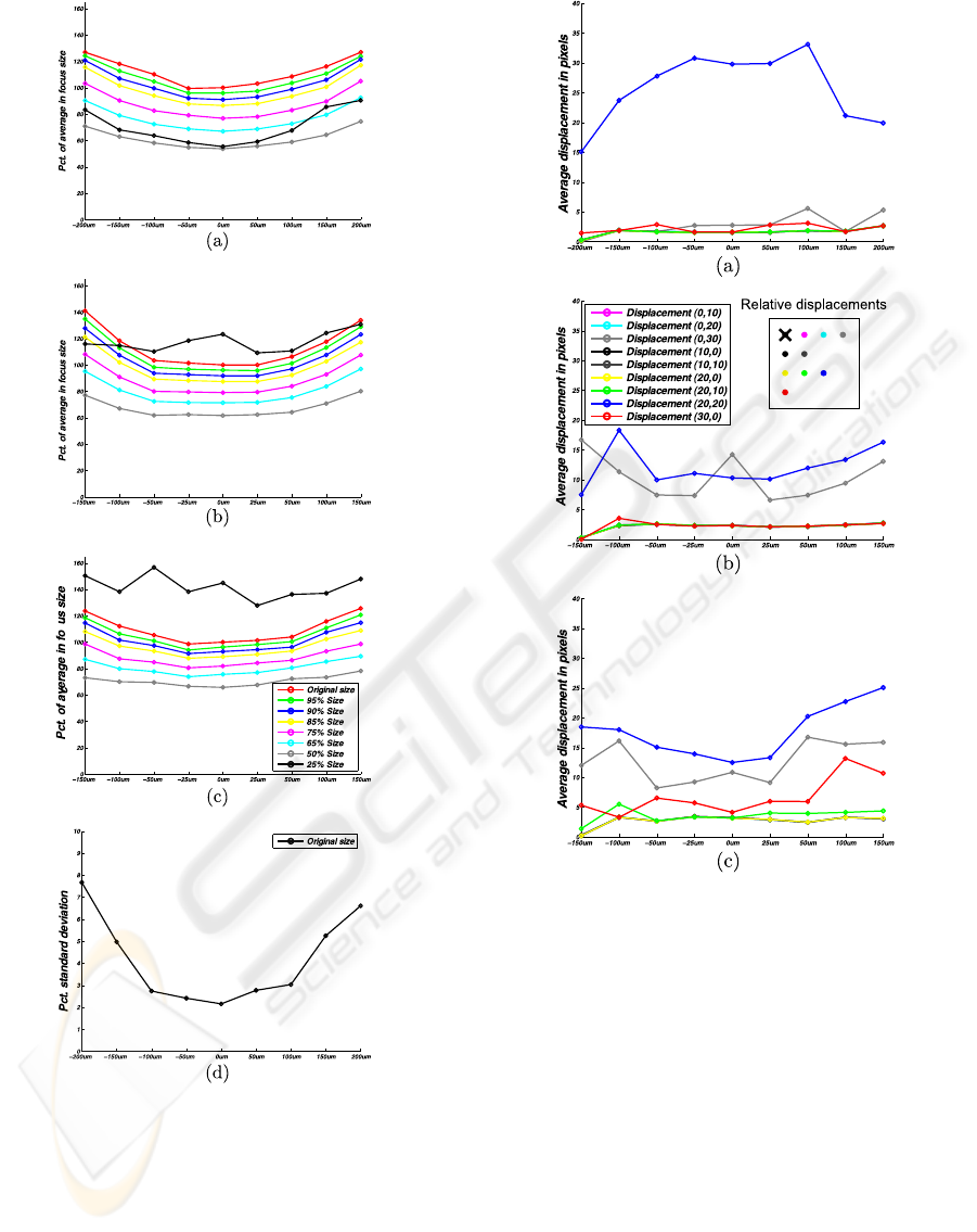
Figure 7: Experiment with change of size. The horizontal

axis of (a)-(c) shows the average radial distance relative to

the in focus particle of original size. Standard deviation of

the size estimate in percent of the original (d). Note the

bias towards overestimation of size and less certainty as a

function of out of focus.

Regression Experiment. Results from our regres-

sion experiment is shown in Table 2. The regression

is performed using ridge regression with λ = 10

−5

We divided our data set into approximately half train-

Figure 8: Experiment for testing robustness to wrong spa-

tial initialization of particle. Vertical axis is the average dis-

tance in pixels to the true position and horizontal axis is the

particle distance to the focus plane. A 50 µm particle has

a radius of about 17 pixels. Experiments have been carried

out for simulated particles, which are spherical (a), ellip-

soids (1 × 2) (b), and ellipsoids (1 × 3) (c). Ellipsoids have

the major axis vertical. The displacements are schemati-

cally shown in (b). Each displacement step is 10 pixels.

ing and half test sets, which was 12 particles from

the simulated set for training and 13 particles for test,

from each image. In the real data set, we have 82 de-

picted particles, and the split was 41 in each group.

We had 27 simulated images, giving 675 observations

for the simulation set. In the observed data set we

have 82 particles in 9 images giving 738 observations.

The results are obtained from 100 random splits in test

and training data. We use the mean radial descriptor

) and the length for each line segment (r

) as input

SHAPE AND SIZE FROM THE MIST - A Deformable Model for Particle Characterization

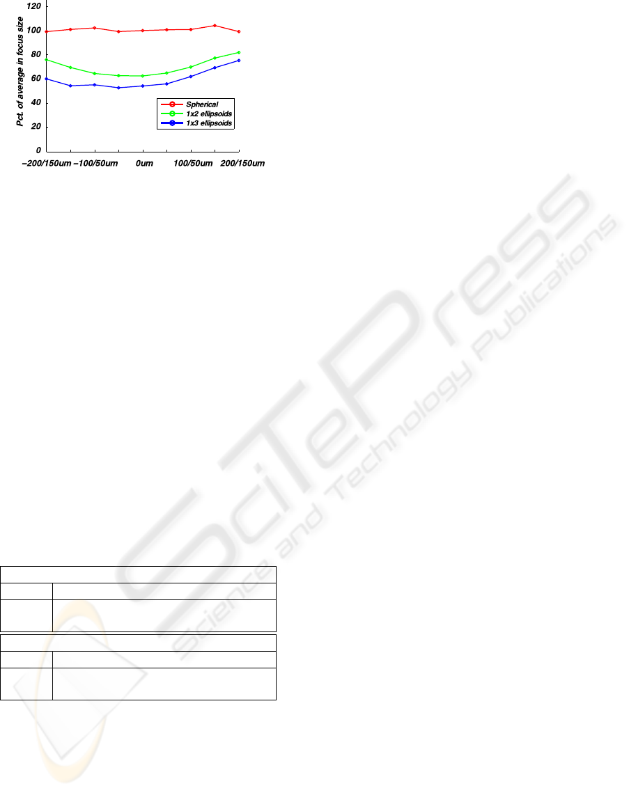
Figure 9: Shape experiment. The horizontal axis is the rela-

tion between the vertical and horizontal line segments from

our particle model, corresponding to the minor and major

axis in the simulated ellipsoids. The true relation for the red

curve would be 1, the green curve would be 0.5 and the blue

curve would be 0.33.

to our regression, see Equation 4.

In the simulated data we perform a regression for

both distance to the focus plane, particle size, and

shape, which is the relation between the major and

minor axis. The obtained results show precise predic-

tions, indicating that this characterization is adequate

for reliable particle modeling. For the real data we

also obtained satisfactory prediction of the distance to

the focus plane, but with about 50% lower precision.

Table 2: Regression model. Regression has been done for

both simulated and real data. There were 25 particles in

the simulated data and 82 particles in the real data set. The

reported numbers are the standard deviation of the absolute

errors of the regression, and the size range of the numbers.

The columns are distance to the focus plane (Distance FP),

average radial line length (Size), relation between the radial

and horizontal line lengths (Shape).

Simulated data

Distance FP Size Shape

Std. 14.20µm 0.8921µm 0.0357

Range 0-200µm 33.3-50µm 0.33-1.0

Real data

Distance FP

Std. 21.69µm

Range 0-180µm

4 DISCUSSION

The data for our experiment is based on LED illumi-

nation, both what is used in the real data, and what

is simulated. This is a rather cheep solution, and if it

can provide satisfactory results, it will be a cost effec-

tive solution. But the rather diffuse illumination from

the LEDs could be replaced by collinear laser, which

will give much higher particle contrast, and therefore

potentially improved performance. Wether this will

give larger depth of ﬁeld or just improved predictions

is for future investigations to show.

The size experiment illustrates how robust our par-

ticle model is to the initialization. With the same set

of parameters, it is capable of handling up to 50%

scale change. But with an initialization, using for ex-

ample scale space blob detection, this should be ade-

quate to adjusting the parameters to obtain a precise

particle characterization.

Scaling images for size variation does not account

for the change i optical properties of smaller particles.

We know that smaller particles in back-illumination

change appearance caused by scattering effects like

refraction and defraction, and this requires further in-

vestigations to verify that our model will be able to

characterize these particles. The appearance change

will result in blurred particles, which our particle

model handles ﬁne. As a consequence the main fo-

cus should be on weather the regression model can

predict the true size. Our regression experiment indi-

cates that this should be possible.

The shape experiment shows that the model does

not adapt precisely to the shape of the particle. This

is caused by the Gaussian noise removal, which also

blurs the particles making them appear less ellipsoid

than they are in reality. The reason for the quite dra-

matic Gaussian convolution, which actually acts con-

trary to the deconvolution that we are trying to infer, is

the noise level in the simulations. The noise is much

larger, than what is seen in the real data, which can be

seen by comparing the images in Figure 5 (c) and Fig-

ure 6 (b). But even with this high noise level, it was

possible to infer the true shape by ridge regression.

Our regression experiment shows that the size,

shape, and distance to the focus plane can be inferred

using our particle model. This is highly encourag-

ing, because it can help in performing more reliable

particle analysis, than by just using the in focus parti-

cles, see e.g. (Ghaemi et al., 2008). The linear ridge

regression is a simple procedure, and much more ad-

vanced methods exists, which for example can han-

dle non-linearities. This might be relevant for infer-

ring particle information of a larger size range or very

small particles, where scattering effects are more pro-

nounced. In this paper we have chosen to primarily

focus on the particle model, so we leave this for fu-

ture investigations.

The data set for our experiments are somewhat

limited, and we plan to extend the data in future in-

vestigations. This should also include less noisy sim-

ulations, which can be obtained from extended sim-

ulation time. In addition to more data, we will also

VISAPP 2010 - International Conference on Computer Vision Theory and Applications

investigate how model parameters can be used for pre-

dicting properties of real data. This will enable simu-

lations of complicated particle modeling for which it

is very hard to obtain ground truth, for example com-

plicated shaped particles or various illumination con-

ditions. From this better analysis setups can be de-

signed, and expected performance can be estimated.

There are no comparative studies between our

model and similar approaches, because other proce-

dures are based on modeling in focus particles, see

e.g. (Fisker et al., 2000; Ghaemi et al., 2008). The ra-

dial sampling lines, which we use in our model, will

give much weight to the center part of the particle.

How this inﬂuences the particle predictions and if this

can help for improvements should be investigated.

5 CONCLUSIONS

There are two main contributions of the work pre-

sented in this paper. Our ﬁrst contribution is that we

experimentally show that out of focus particles can be

modeled reliably, and therefore be included in obtain-

ing information of particle size, shape and distance to

the focus plane. This is enabled through our particle

model, which is our second contribution. The model

is very robust and provides precise predictions of par-

ticle characteristics. We hope that this can help in re-

moving some of the mist from particle characteriza-

tion, and hereby give better performance and system

design to particle analysis in the future.

ACKNOWLEDGEMENTS

This work has been partly ﬁnanced by the EU-project

PROVAEN under the Sixth Framework

. We also

thank our collaborators from Dantec A/S

for provid-

ing data and fruitful discussions.

REFERENCES

Cho, S., Matsushita, Y., Lee, S., and Postech, P. (2007).

Removing non-uniform motion blur from images. In

IEEE 11th International Conference on Computer Vi-

sion, 2007. ICCV 2007, pages 1–8.

Dai, S. and Wu, Y. (2008). Motion from blur. In Proc. Conf.

Computer Vision and Pattern Recognition, pages 1–8.

http://www.provaen.com/

http://www.dantecdynamics.com/

Fisker, R., Carstensen, J. M., Hansen, M. F., Bødker, F., and

Mørup, S. (2000). Estimation of nanoparticle size dis-

tributions by image analysis. Journal of Nanoparticle

Research, 2(3):267–277.

Ghaemi, S., Rahimi, P., and Nobes, D. (2008). Measure-

ment of Droplet Centricity and Velocity in the Spray

Field of an Effervescent Atomizer. Int Symp on Appli-

cations of Laser Techniques to Fluid Mechanics, Lis-

bon, Portugal, 07-10 July, 2008.

Hastie, T., Tibshirani, R., Friedman, J., and Franklin, J.

(2005). The elements of statistical learning: data min-

ing, inference and prediction. The Mathematical In-

telligencer, 27(2):83–85.

Kundur, D. and Hatzinakos, D. (1996). Blind image decon-

volution. IEEE signal processing magazine, 13(3):43–

64.

Levin, A. (2007). Blind motion deblurring using image

statistics. Advances in Neural Information Processing

Systems, 19:841.

Lindeberg, T. (1994). Scale-space theory in computer vi-

sion. Springer.

Lucy, L. B. (1974). An iterative technique for the recti-

ﬁcation of observed distributions. The astronomical

journal, 79(6):745–754.

Narayan, R. and Nityananda, R. (1986). Maximum entropy

image restoration in astronomy. Annual review of as-

tronomy and astrophysics, 24(1):127–170.

Richardson, W. H. (1972). Bayesian-based iterative method

of image restoration. Journal of the Optical Society of

America, 62(1):55–59.

Shan, Q., Jia, J., and Agarwala, A. (2008). High-quality

motion deblurring from a single image. ACM Trans-

actions on Graphics-TOG, 27(3):73–73.

Shan, Q., Xiong, W., and Jia, J. (2007). Rotational mo-

tion deblurring of a rigid object from a single image.

In IEEE 11th International Conference on Computer

Vision, 2007. ICCV 2007, pages 1–8. Citeseer.

Starck, J. L., Pantin, E., and Murtagh, F. (2002). Decon-

volution in astronomy: a review. Publications of the

Astronomical Society of the Paciﬁc, 114(800):1051–

1069.

Wiener, N. (1964). Extrapolation, Interpolation, and

Smoothing of Stationary Time Series. The MIT Press.

SHAPE AND SIZE FROM THE MIST - A Deformable Model for Particle Characterization