TWO DOF CAMERA POSE ESTIMATION WITH A PLANAR
STOCHASTIC REFERENCE GRID
Giovanni Gherdovich and Xavier Descombes
INRIA Sophia Antipolis, 2004 route des Lucioles, Sophia Antipolis, France
Keywords:
Camera pose estimation, Shape from texture, Poisson point process, Posson-Voronoi tessellation.
Abstract:
Determining the pose of the camera is a need to many higher level computer vision tasks. We assume a set
of features to be distributed on a planar surface (the world plane) as a Poisson point process, and to know
their positions in the image plane. Then we propose an algorithm to recover the pose of the camera, in the
case of two degrees of freedom (slant angle and distance from the ground). The algorithm is based on the
observation that cell areas of the Voronoi tessellation generated by the points in the image plane represent
a reliable sampling of the Jacobian determinant of the perspective transformation up to a scaling factor, the
density of points in the world plane, which we demand as input. In the process, we develop a transformation
of our input data (areas of Voronoi cells) so that they show almost constant variances among the locations, and
analytically find a correcting factor to considerably reduce the bias of our estimates. We perform intensive
synthetic simulations and show that with few hundreds of random points our errors on angle and distance are
not more than few percents.
1 INTRODUCTION
With “camera pose estimation” one refers to the prob-
lem of determining the position and orientation of a
photo camera with respect to the coordinate frame of
the imaged scene. When acquiring this information
by external instruments is too expensive for the ap-
plication of interests, or simply is impossible because
the picture is already taken, one must resort to com-
puter vision techniques and use at best the visual data
at disposal. It is a task that needs to be performed
in a wide range of different situations, subsumed by
many higher level computer vision problems like ob-
ject detection, object recognition, vision-based safety
applications, augmented reality. Anytime one needs
to measure metric or affine quantities in a 3D scene
captured by a photo camera, the parameters of the
perspectiveprojection need to be recovered, i.e. infor-
mation about the camera position have to be inferred
from the image itself.
In the case the images containing artifacts like
buildings or other non-natural structures, classical ap-
proaches consist in finding straight lines, known an-
gles, orthogonalities or reference points and use them
to invert partially or totally the perspective distor-
tion (Hartley and Zisserman, 2004). Images of nat-
ural scenes don’t offer such references, and other ap-
proaches need to be investigated. In recent years, re-
searchers have proposed approaches that leverage the
statistical properties of the viewed scene. The main
idea is to study how these properties are modified in
the image by the perspective distortion, so that the
desired information about the parameters of the per-
spective itself can be estimated. Shape from texture
is a well established techniques that uses the perspec-
tive distortion of some homogeneous or isotropic pat-
tern to get 3D clues about a surface shape (Permuter
and Francos, 2000), (Malik and Rosenholtz, 1997),
(Clerc and Mallat, 2002), (G˚arding, 1992), (Kanatani
and Chou, 1989).
Although the problem of estimating the position
and orientation of the camera has received a consider-
able amount of attention, little has been done in esti-
mating the camera pose using features uniformly dis-
tributed in a picture. Our approach leverages some
of the intuitions foundational to shape from texture
techniques; namely we use the concept of area gra-
dient (G˚arding, 1992) to determine the nature of the
perspective transform. The main objective is to ex-
ploit the information content of the location of uni-
formly distributed features, which can actually come
from preprocessing homogeneous image textures, but
they can also correspond to the spatial locations of
objects whose background is not a homogeneous tex-
179
Gherdovich G. and Descombes X. (2010).
TWO DOF CAMERA POSE ESTIMATION WITH A PLANAR STOCHASTIC REFERENCE GRID.
In Proceedings of the International Conference on Computer Vision Theory and Applications, pages 179-184
DOI: 10.5220/0002828501790184
Copyright
c
 SciTePress

ture. This differentiates with the shape from texture
paradigm which relies on the presence of homogene-
ity or isotropy on a whole patch of the image. There-
fore, the information embedded in the image required
to estimate the camera pose is lesser, leading to a
wider application area. Because of those reasons in
the present work we suggest the decoupling, in the
spirit of (Kanatani and Chou, 1989), between image
processing and distortion analysis in the task of re-
covering the orientation of a planar surface subjected
to perspective transformation.
In this paper we assume the viewed scene to be
a planar surface on which a Poisson point process
takes place, i.e. the points are uniformly distributed
on such “world plane”; our technique first measures
the perspective distortion induced on this pattern by
the transformed size of small areas surrounding each
point in the resulting image. Then this measure is
linked to the parameters of the perspective transfor-
mation we’re interested in, i.e. the slant angle and
the distance from the scene along the optical axis. In
particular, we model the intuitive concept of “small
areas” using the size of the cells in the Voronoi tes-
sellation generated by the point pattern. We do that
through the following observation: the size of the
Voronoi cell centered at the point p in the image di-
vided by the size of a typical cell of the Poisson-
Voronoi tessellation in the world plane yields a rea-
sonable approximation of the Jacobian determinant
of the perspective transform computed in the back-
image of the point p. Our simulations confirm this
intuitive claim: with this procedure, given the density
λ of the Poisson process we get consistent estimation
for the slant angle and the distance from the ground.
The main contribution of this work is the tailor-
ing of the area gradient concept to the case of a dis-
crete set of points through the use of Voronoi tessel-
lations. In the process, we develop a transformation
of our input data (areas of Voronoi polygons) so that
they show almost constant variances among the dif-
ferent locations in the image plane, and analytically
find a correcting factor for the linear model to which
we fit such data in order to have an unbiased linear
least squares estimation of the parameters of interest,
slant angle and distance.
The remaining of the paper is organized as fol-
lows: in Section 2 we present the homographywe will
consider during the subsequent sections; in Section 3
we define formally the problem, then we introduce
our algorithm in Section 4 and present the results of
our experiments in Section 5. Our conclusions will be
given in Section 6.
2 THE HOMOGRAPHY UNDER
STUDY
In this work we consider homographies between
planes, i.e. our perspective transformation, induced
by an ideal pinhole camera, will be a function P :
P
2
→ P
2
where P
2
is the projective plane; P is repre-
sented in homogeneous coordinates by a 3×3 matrix,
defined up to a multiplicative factor. We name world
plane the domain of P, and image plane its codomain.
The principal ray is the line from the camera center
perpendicular to the image plane and the principal
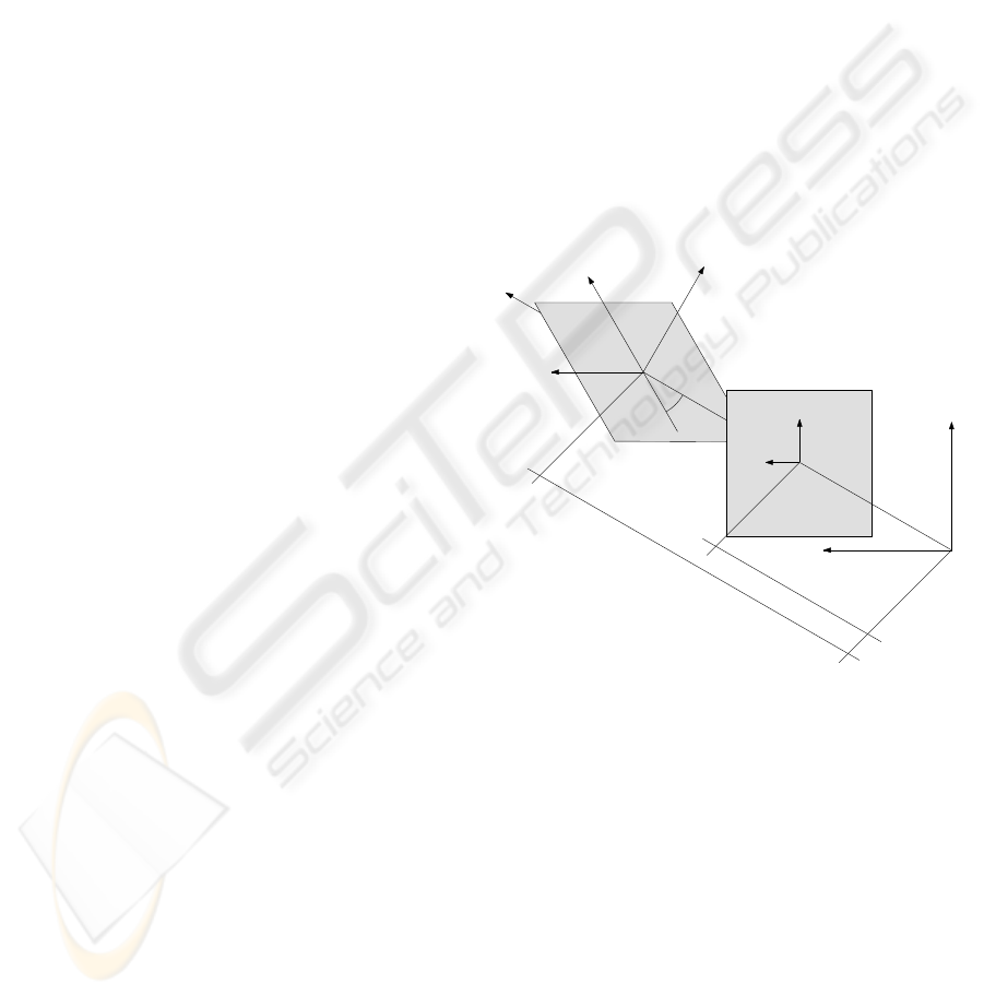
point is its intersection with the image plane. In a
completely general settings, we have eight degrees of
freedom (DOF) over P; we restrict our attention to the
case of two DOF, namely the distance d between the
camera center and the inverse image of the principal
point through P, and the angle θ between the principal
ray and the world plane (see figure 1). The remaining
y
x
u
v
image plane
world plane
f
d
theta
camera center
Figure 1: Camera center, image plane and world plane.
parameters are reference frames for the two coordi-
nate systems and orientation of the world plane with
respect to the image plane, and they are chosen in or-
der to send the vanishing line of the world plane to an
horizontal line in the image; the focal length f is as-
sumed to be known, the pixels are squared and there
is no skew.
Let us consider the origins of the world and image
coordinate systems are the inverse image of the prin-
cipal point and the camera center respectivelythen ex-
pression of P is the following:
P : P
2
−→ P
2


u
v
w


7−→


f 0 0
0 f sinθ 0
0 cosθ d




u
v
w


(1)
VISAPP 2010 - International Conference on Computer Vision Theory and Applications
180

For the sake of clarity we remark its behavior on
the affine part:
P
d,θ
(u,v) = (x(u, v),y(u,v)) (2)
=

uf
vcosθ+ d
,
vf sinθ
vcosθ+ d

3 PROBLEM STATEMENT
Suppose that a certain number of points are uniformly
distributed on some portion of the world plane, and
that we look at them through our pinhole camera,
whose model is described in Section (2). Then, their
spatial distribution is not uniform anymore in the im-
age plane. We assume to have some good algorithm
to detect their position in the picture, and our aim is to
recover the parameters d and θ of the planar homogra-
phy studying such distortion. As stated in Section (2)
the “horizon” is assumed to be parallel to the horizon-
tal axes of the image, but it can be very well outside
the picture. In our framework, the density of points λ
in the world plane (i.e. the number of points per unit
area) needs to be known — it’s a consequence of the
formula (2), where P
ds,θ
(us,vs) = P
d,θ
(u,v) for every
s ∈ R, which means that changing the distance d is
equivalent to change scale in the world plane, and just
looking at the picture we cannot distinguish between
small distance with dense points and big distance with
sparse points.
4 THE ALGORITHM
In order to study the perspective distortion of uni-
formly distributed points, one need to capture the fol-
lowing intuitive notion: points get closer to each other
as approaching to the horizon. What is needed is a
statistical quantity able to discriminate between dif-
ferent perspective projections; our suggestion is to
measure “how much free space” S
p
is present around
each point p of our random configuration. Suppose
that we were able to know S
p
in the world plane for a
given p, and also its transformation, denoted by abuse
of notation P(S
p
); if S
p
was small enough, i.e. if
the points where sufficiently dense, the ratio of ar-
eas |P(S
p
)|/|S
p
| would have been a good estimation
of the determinant of the Jacobian matrix of P at the
point p — the Jacobian determinant measures the fac-
tor with which a function modifies volumes around a
point. And doing this for all the points of the config-
uration, one can have many samples of the Jacobian,
hopefully enough to do a regression and estimate the
parameters of interest d and θ.
But what does “free space around a point” means?
And what is |S
p
|? We don’t have any clue about the
world plane, we just have its perspective view. Again:
what is P(S
p
)? We don’t even know the function P.
A reasonable answer to the first question is given
by the 2-dimensional Voronoi diagram, a tessellation
of the plane generated by a set of points {p
i
} such
that a point q belongs to the cell of p
k
if it’s closer to
p
k
than to any other p
i
; small Voronoi cells mean that
the generating points are “dense”. So for us the free
space around a point is its Voronoi cell. The answer
to the second question is 1/λ, where λ is the density
of points in the world plane. In fact, this is the ex-
pected value for |S
p
|, assuming a Poisson distribution
for the points (Hayen and Quine, 2002); the key point
is its independence from p, which can be intuitively
understood observing that if we take some region A
in the world plane, the expected value of the num-
ber of points inside A is proportional to the area of
A, no matter of its location. In the third question we
ask how to approximate the projection of the Voronoi
cell S
p
; our answer is to compute the Voronoi diagram
generated by the projected points.
Before stating precisely our algorithm we write
the formula of the Jacobian determinant (from now on
just “Jacobian”) of our homography, using the same
notation as in eq. (2)
J
P
(u,v) = det

x
u
x
v
y
u
y
v

=
f
2
d sinθ
(vcosθ+ d)
3
(3)
and point out that since all our measurements are done
in the image plane, while the domain of the above Ja-
cobian is the world plane, what we are going to sam-
ple is the composition
(J
P
◦P
−1
)(x,y) =
( f sinθ−ycosθ)
3
f(d sinθ)
2
(4)
= (a+ yb)
3
At this point, the natural choice to recover the pa-
rameter a and b, hence d and θ, would be to set the
linear regression model
λ|P(S
p
)| = (a+ by)
3
+ ε (5)
where the zero mean noise is taken into account by
the random variable ε. Unfortunately, the variance of
ε varies with the location of the cell S
p
; furthermore,
it is reasonable to assume that such variance is trans-
formed under perspective likewise areas, i.e.
Var(ε) = (λ(a+ by)
3
)
2
Var(S
p
) (6)
This means that knowing Var(ε) is equivalent to know
the parameters a and b that we’re about to estimate.
Any heuristic we could use to estimate the variances
of the errors ε will result in a poor fitting to the 3rd
TWO DOF CAMERA POSE ESTIMATION WITH A PLANAR STOCHASTIC REFERENCE GRID
181

degree polynomial (4); also, in weighting the least
squares summation with empirical variances we ex-
perimented numerical problems due to very small
condition numbers of the matrices involved. For this
reason we resort to a variance-stabilizing transfor-
mation; by the error propagation formula (G.Cowan,
1998) and given the assumption (6), the ideal can-
didate would be the logarithm, but the regression
wouldn’t be linear any more. We found experimen-
tally that the cube root of our data {λ|P(S
p
)|}
p
shows
approximately constant variances.
Thus we don’t use model (5) for our regression,
but
3
q
λ|P(S
p
)| = (a+ by) + η (7)
With a second order Taylor expansion of the left-
hand-side around (a+by)
3
one can show that E(η) =
−λ
2
(a + by)Var(S
p
)/9 —interestingly, the mean of
the noise is proportional to a + by. A closed form
for the variance Var(S
p
) of cell sizes for a Poisson
Voronoi tessellation is not known, but the six decimal
digits approximation 0.280176/λ
2
found in (Hayen
and Quine, 2002) is more than enough for our pur-
poses. Thus we can restate (7) in a suitable form for
the ordinary least squares method, i.e. with an error
term
˜
η that has zero mean and constant variance:
3
q
λ|P(S
p
)| = (a+ by)

1−
0.280176
9

+
˜
η (8)
What follows is the detailed algorithm we use.
1. INPUT: the points {p
1
,..., p
n
} in the image
plane.
2. Generate the Voronoi diagram from {p
1
,..., p
n
}.
3. Points close to the boundaries of the viewed scene
will produce degenerate cells, i.e. unbounded or
very oblong. Remove all the cells which have at
least one vertex outside the viewed scene.
4. Compute the areas of the remaining cells
{C
1
,...,C
k
}, where C
i
is the cell generated by the
point p
i
(we reordered the cells so that the first
k are the ones we keep). These are k noisy sam-
ples of the function J
P
◦P
−1
up to the (known)
scaling factor λ, in the sense that area(C
i
) ≈ J
P
◦
P
−1
(p
i
)/λ.
5. Solve the linear least squares problem
min
a,b
∑
i

3
p
λ area(C
i
) −(a+y
i
b)

1−
0.280176
9

2
(9)
where y
i
is the y-coordinate of the point p
i
.
6. OUTPUT: the estimates
ˆ
θ = arctan

−a
fb

ˆ
d =
f
a
4
√
b
2
f
2
+a
2
(10)
5 EXPERIMENTAL RESULTS
We evaluated our algorithm on a set of random point
configurations synthetically generated; the parame-
ters of interest that we vary are the slant angle θ of
the camera and the number of points in the config-
uration; we keep fixed the length d of the principal
ray to 100 meters. We recall that at a given θ, adding
points to the configuration while keeping d constant
is equivalent to keep the point density constant and
increase d. We tested the algorithm with 12 angles θ
ranging uniformlyfrom 2
◦
to 60
◦
and with the number
of points ranging uniformly from 100 to 2000; for ev-
ery of these combinations we generated one hundred
random point configurations. During the simulation
we kept the focal length f fixed to 50mm, and our
pictures are squares of 25mm×25mm centered in the
origin of the image plane.
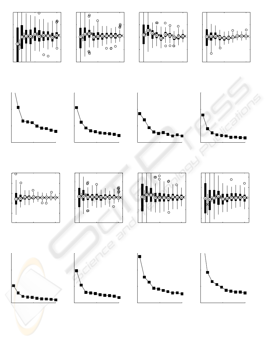
Figure 2 reports our results concerning the esti-
mation of the distance d. It shows 4 plots, corre-
sponding to some of the values of θ for which we
tested the algorithm. Each plot contains columns rep-
resenting a boxplot and a 95% confidence interval for
ten different quantities of points in the image, from
100 to 2000. For every of these quantities we simu-
lated 108 different point patterns; the boxplots sum-
marize those measures, with median, lower and up-
per quartile, maximum and minimum observed value,
outliers. The confidence interval on the right of each
boxplot refers the empirical mean E(
ˆ
d) and is based
on the Student’ t distribution. Figure 3 is closely re-
lated to figure 2, since it shows the relative errors of
the empirical mean |E(
ˆ
d) −d|/d, where d is the true
value and
ˆ
d the estimator. The first information these
two figures show is that as the number of points in-
creases, our estimator gets more accurate: the vari-
ability in figure 2 decreases towards the right hand
side, the confidence intervals get narrower and the rel-
ative error resembles loosely a multiple of the inverse
of the square root of the number of points. We per-
formed tests up to 5000 points, and the results show
and improved convergence, but we consider unrealis-
tic the demand for more than 2000 feature points in
the scene. The same holds for the estimator of the
slant angle
ˆ
θ, figures 4 and 5. As a rule of thumb, we
can say that with at least 1000 points in the image we
can get reliable estimates of slant and distance (less
than 5% of error).
6 CONCLUSIONS
In this work we propose a novel technique to study the
distortion induced by perspective projection on a pla-
VISAPP 2010 - International Conference on Computer Vision Theory and Applications
182

100 1000 2000
80
90
100
110
120
theta = 13°
100 1000 2000
80
90
100
110
120
theta = 28°
100 1000 2000
80
90
100
110
120
theta = 44°
100 1000 2000
80
90
100
110
120
theta = 60°
Figure 2: Estimated distance versus number of points.
0 1000 2000
0
5
10
15
theta = 13°
0 1000 2000
0
5
10
15
theta = 28°
0 1000 2000
0
5
10
15
theta = 44°
0 1000 2000
0
5
10
15
theta = 60°
Figure 3: Relative error for
ˆ
d versus number of points.
100 1000 2000
11
12
13
14
15
theta = 13°
100 1000 2000
24
26
28
30
32
34
theta = 28°
100 1000 2000
40
45
50
theta = 44°
100 1000 2000
50
55
60
65
70
theta = 60°
Figure 4: Estimated slant angle θ versus number of points.
0 1000 2000
0
5
10
15
theta = 13°
0 1000 2000
0
5
10
15
theta = 28°
0 1000 2000
0
5
10
15
theta = 44°
0 1000 2000
0
5
10
15
theta = 60°
Figure 5: Relative error for
ˆ
θ versus number of points.
nar Poisson point process; we use this to recover the
pose of a pinhole camera with two degrees of free-
dom, slant angle and distance from the ground along
the optical axis. Our approach relies on the observa-
tion that the Voronoi tessellation generated by a Pois-
son point process under perspective is a faithful rep-
resentation of the area transformation ratio, i.e. the
Jacobian of the perspective, up to a scaling factor that
we demand as input (the density of the Poisson pro-
cess). We perform intensive simulations on synthetic
data and do a careful error analysis, concluding that
1000 points on the scene are enough to get estimates
of the parameters of interests with an error less than
5%. Our work borrows ideas from the shape from tex-
TWO DOF CAMERA POSE ESTIMATION WITH A PLANAR STOCHASTIC REFERENCE GRID
183

ture paradigm (the area gradient concept), but instead
of assuming the presence of a whole patch of homoge-
neous or isotropic texture, we pursue a feature-based
approach which considers only a discrete set of points
with homogeneity properties; such different premises
make a direct comparison with shape from texture al-
gorithms non obvious. Our hypothesis make the pro-
posed solution more suitable for camera pose estima-
tion in general settings, specifically natural environ-
ments, where reference artifacts are missing and one
must resort to stochastic modeling.
ACKNOWLEDGEMENTS
The authors would like to thank Jean-Denis Durou,
Ian Jermyn, Giovanni Neglia and Roberto Cascella
for many useful discussions that improved consis-
tently the shape of this article.
REFERENCES
Clerc, M. and Mallat, S. (2002). The texture gradient equa-
tion for recovering shape from texture. IEEE Trans-
actions on Pattern Analysis and Machine Intelligence,
24(4):536–549.
G˚arding, J. (1992). Shape from texture for smooth curved
surfaces in perspective projection. Journal of Mathe-
matical Imaging and Vision, 2:329–352.
G.Cowan (1998). Statistical Data Analysis. Oxford Univer-
sity Press.
Hartley, R. and Zisserman, A. (2004). Multiple View Geom-
etry in Computer Vision. Cambridge University Press,
2nd edition.
Hayen, A. and Quine, M. P. (2002). Areas of components of
a voronoi polygon in a homogeneous poisson process
in the plane. Adv. Appl. Probab, 34:281–291.
Kanatani, K. and Chou, T. (1989). Shape from texture: Gen-
eral principle. Artificial Intelligence, 38:1–48.
Malik, J. and Rosenholtz, R. (1997). Computing local sur-
face orientation and shape from texture for curved
surfaces. International Journal of Computer Vision,
23(2):149–168.
Permuter, H. and Francos, J. M. (2000). Estimating
the orientation of planar surfaces: Algorithms and
bounds. IEEE Transactions on Information Theory,
46(5):1908–1920.
VISAPP 2010 - International Conference on Computer Vision Theory and Applications
184