THE SONG PICTURE

On Musical Information Visualization for Audio and Video Editing

Marcelo Cicconet and Paulo Cezar Carvalho

Vision and Graphics Laboratory, IMPA, Rio de Janeiro, Brazil

Keywords:

Musical information visualization, Chroma vector, Loudness, Self-similarity matrix, Novelty score.

Abstract:

Most audio and video editors employ a representation of music pieces based on the Pulse Code Modulation

waveform, from which not much information, besides the energy envelope, can be visually captured. In

the present work we discuss the importance of presenting to the user some hints about the melodic content

of the audio to improve the visual segmentation of a music piece, thereby speeding up editing tasks. Such

a representation, although powerful in the mentioned sense, is of simple computation, a desirable property

because loading an audio or video should be done very fast in an interactive environment.

1 INTRODUCTION

When working with audio or video edition, it is natu-

ral, if not mandatory, to use the visual representation

of the audio track provided by the software as a rough

guide to the onset or offset point of the media chunk

that has to be edited.

To the best of our knowledge, all general purpose

software for audio and video editing make the sound

track visible by presenting its Pulse Code Modulation

(PCM) waveform.

Supposing the audio is mono-channel (in other

cases, all channels can be mixed down to just one),

the PCM representation is simply the graph of times-

tamp versus amplitude, where the samples are taken

at equally spaced time intervals, normally at a sam-

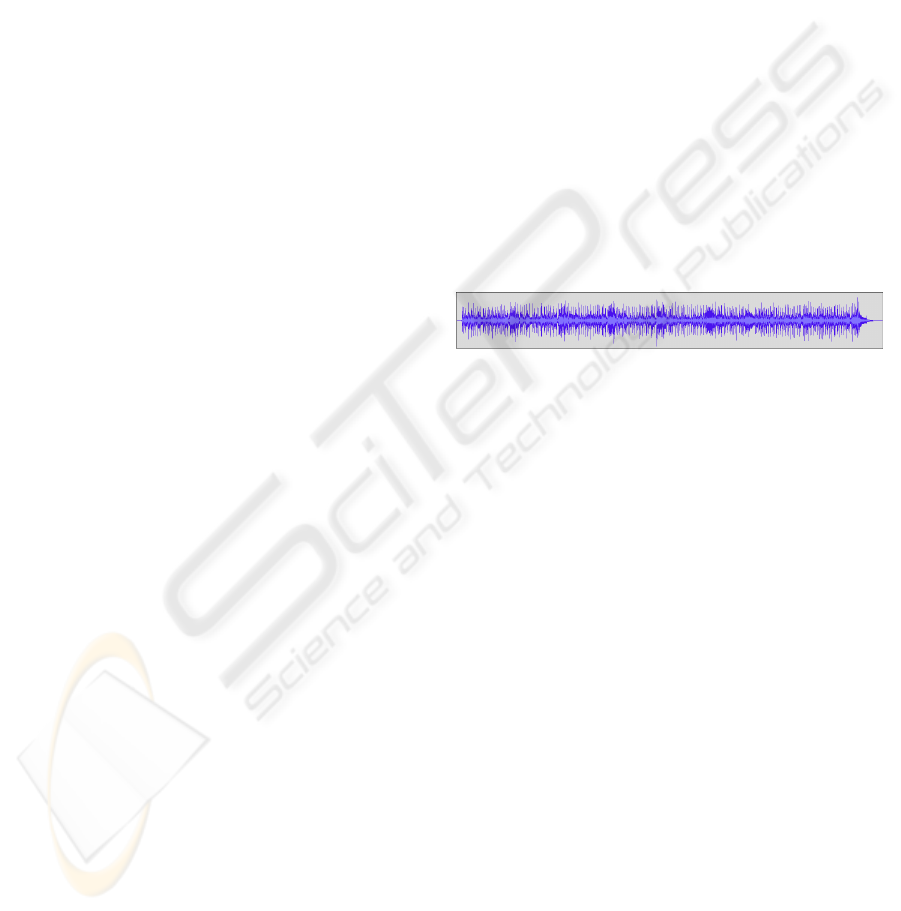
ple rate of 44100 samples per second. Figure 1 shows

an example. The value represented is simply “raw”

sound, the Sound Pressure Level (SPL) as it would be

measured by a microphone.

In the example shown by Figure 1 it is difﬁcult to

point out boundaries of regions with distinct musical

content, where by distinct musical content we mean

an obvious audible dissimilarity between the region

located before and the region located after a speciﬁc

point in time.

This problem is less evident if the predominant

musical information in the audio ﬁle is percussive

(like in drum sequences, for example). However, ﬁrst

of all the great majority of song ﬁles have relevant

melodic content, and furthermore even percussive in-

struments can be classiﬁed as of low or high pitch, a

Figure 1: Audio PCM representation of a song synthesized

by Garage Band, as shown by Audacity.

melodic property.

The main goal of this work is to show that the

melodic content of an audio ﬁle is worth noting when

implementing visualizers of entire music pieces in au-

dio and video editors. We claim that by using the

low level audio descriptors of loudness and chroma,

to be deﬁned below, we can build a representation of

the audio ﬁle which, on the one hand, resembles the

waveform, and on the other hand, gives more hints

about adjacent regions of the audio ﬁle with different

musical content.

The rest of the paper is as follows. In section 2

we will talk about what can be found in the litera-

ture on this subject. Section 3 describes our proposed

mapping between audio and visual content. We will

deﬁne the above mentioned low level descriptors, as

well as discuss some constraints (especially regarding

computational cost) that have guided the choice of the

method. In section 4 we will be concerned with the

question of evaluating the method. Some strategies

will be mentioned, and our choices will be justiﬁed.

Section 5 is the place for results, lined by the con-

clusions of section 4. This text ends with some ﬁnal

remarks in section 6.

Cicconet M. and Cezar Carvalho P. (2010).

THE SONG PICTURE - On Musical Information Visualization for Audio and Video Editing.

In Proceedings of the International Conference on Imaging Theory and Applications and International Conference on Information Visualization Theory

and Applications, pages 85-90

DOI: 10.5220/0002825000850090

 SciTePress

Figure 2: Loudness and Chroma features of a 30 seconds long portion of the song Anything Goes, by ACDC. The features

are extracted from windows with 4096 frames, and the overlap is of 2048 frames. The audio sample rate is of 44100 frames

per second.

2 RELATED WORK

When speaking about audio visualization, it is worth

clarifying what sort of visualization is being treated.

We can mention at least three cases where terms like

music visualization or audio visualization apply.

First, there are the online visualization algorithms.

They show in real-time (or at least as real-time as pos-

sible) some feature extracted from a small window

around the audio portion being played or sung. The

purpose of this kind of visualizer can be of aesthetic

nature, enhancing audio playback software (Lee et al.,

2007), as a tool for musical training (Ferguson et al.,

2005), as a help for the hearing impaired, enhanc-

ing the awareness of their surroundings (Azar et al.,

2007), or as an interface to control real-time compo-

sition parameters (Sedes et al., 2004).

Second, in works like (Kolhoff et al., 2006), a pic-

ture representing the entire audio ﬁle is rendered with

the purpose of facilitate the search in large databases

or simply as a personalized icon of the ﬁle. In (Ver-

beeck and Solum, 2009) the goal is to present a high

level segmentation of the audio data in terms of intro,

verse, chorus, break, bridge and coda, the segments

being arranged as concentric rings, the order from the

center being the same of the occurrence of that part of

the music in the piece.

Finally, there are the methods aiming at rendering

a picture (matrix) of the entire ﬁle in which at least

one dimension is time-related with the audio. Perhaps

the most important example is (Foote, 1999), where

a square matrix of pairwise similarity between small

consecutive and overlapping audio chunks is com-

puted. (We will come back to this kind of matrix later,

in section 4.) Another very common example consist

of plotting time against some 1- or n-dimensional au-

dio feature, like, say, the magnitudes of the Discrete

Fourier Transform coefﬁcients of the audio chunk.

For n-dimensional features the resulting matrix is nor-

malized so that the minimum value is 0 and the max-

imum 255, resulting in a grayscale image. Figure 2

shows this kind of plot in the case of the loudness (1-

dimensional) and chroma (12-dimensional) features.

3 PROPOSED METHOD

The musical content of a piece can be essentially di-

vided in two categories: the harmonic (or melodic)

and the rhythmic (or percussive). Rigorously speak-

ing it is impossible to perform such a division, since

melody and rhythm are (sometimes strongly) corre-

lated. There are, however, ways to extract most of the

content of one or another category, which is the main

issue in the Musical Information Retrieval commu-

nity. The problem with these methods is that they are

usually computationally expensive. In fact, in a pre-

vious work (Cicconet and Carvalho, 2009) we have

tried to segment the music piece and to perform some

kind of clustering. But good clustering requires high

computational cost. This means that the user has to

wait a long time for the result, which is not desirable.

Thus, we decided to use two simple audio de-

scriptors, each one related with a different component

of the audio (rhythm or melody), and combine them

in such a way that the corresponding visual features

complement each other.

Another important point behind this decision re-

lies on the segmentation and clustering capabilities of

the human visual system. It consists of billions of

neurons working in parallel to extract features from

every part of the visual ﬁeld simultaneously (Ware,

2004).

Therefore, instead of spending computational

time segmenting and clustering the audio data, we

moved to the direction of taking advantage of the hu-

man visual capabilities in doing that, and facilitating

the analysis by presenting signiﬁcative audio informa-

tion.

The visualization algorithm we propose is as fol-

lows.

We assume that the audio ﬁle is mono-channel and

sampled at 44100 frames per second; otherwise we

apply some processing (adding the channels and/or

resampling) to obtain audio data with the desired fea-

tures. These properties are not critical; the computa-

tions could be done for each channel separately and

the sample rate could be a different one.

At regular intervals of 2048 frames, an audio

chunk of length 4096 frames is multiplied by a Hann

window, and the Discrete Fourier Transform (DFT) of

it is computed. We choose 2048 as hop size to obtain

IVAPP 2010 - International Conference on Information Visualization Theory and Applications

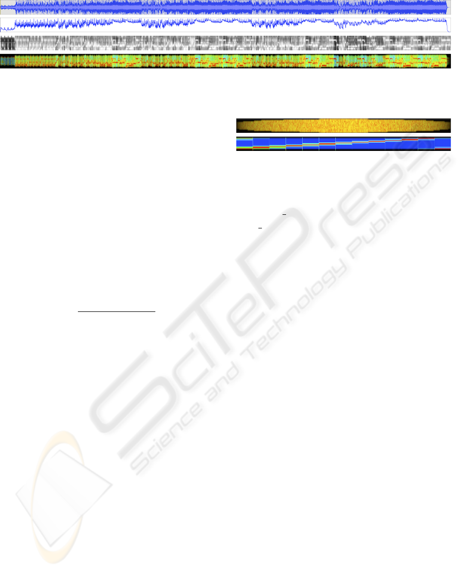
Figure 3: PCM waveform (top), loudness, chroma and the representation described in section 3 of the song Sex on Fire, by

Kings of Leon. In this example, besides the many segmentation points presented, it is also possible to guess what portions of

the picture corresponds to the chorus of the song.

good resolution of feature extraction even for songs

with high tempo (say, 200 beats per second). Also,

the window size of 4096 allows good precision in es-

timating the energy of the waveform corresponding to

low frequencies (those bellow 100Hz).

The loudness audio descriptor was chosen to rep-

resent the rhythm. Loudness is the average of the

magnitudes of the DFT coefﬁcients, a measure highly

related with the energy of the audio, which usually

has a good response to bass and snare drums, and

also resembles the PCM representation, making fa-

miliar the visualization we are describing. The vector

of loudness values is then normalized to fall in the

range [0,1], and warped logarithmically according to

the equation

x →

log(x + c) − log c

log(1 + c) − log(c)

where c > 0 is an offset parameter. (The results pre-

sented here were obtained using c = 0.1.) The log-

arithmic warp is important because the human audi-

tory and visual systems are roughly logarithmically

calibrated.

As melody feature we use the chroma vector, as

described in (Jehan, 2005). First, the magnitudes of

the DFT coefﬁcients, after normalization, are warped

logarithmically as expressed above, then the 84 am-

plitudes corresponding to MIDI notes ranging from

24 to 107 are captured and a 12-dimensional vector

is obtained by summing the amplitudes correspond-

ing to musical notes of the same key in different oc-

taves. The elements of this vector are normalized to

the range [0,1], to avoid taking into account differ-

ences of loudness in different windows, and squared,

to give more importance to the peak value, highlight-

ing the melodic line. Chroma vectors roughly rep-

resent the likelihood of a musical note (regardless of

its octave) being present in the audio window under

analysis.

We arrange the chroma vectors c = (c

,...,c

) as

columns side by side in a matrix, the bottom corre-

sponding to the pitch of C. The entries of each vector

are associated with a color (h,s,v) in the HSV color

space, where the value c

controls the hue component

Figure 4: Algorithm described in section 3 applied to a

faded-in and -out white noise sample (top) and to a C-

through-C 13-notes glissando (bottom).

h as follows: supposing the hue range is [0, 1], we

make h =

(1 − c

), so the color ranges from blue

(h =

) to red (h = 0), linearly, when c

ranges from 0

to 1. We set s = 1 and v = l

, where l

is the loudness

value corresponding the chroma vector c.

Each vector (column) is then warped vertically (in

the sense of image warping), having the middle point

as pivot. The warping is such that the height h

of the

vector ranges from α to 2α, where α is some positive

constant not smaller then 12 pixels. More precisely,

is given by h

= (1 + l

)α.

Figure 3 shows our method at work. The wave-

form, as well as the audio features used to build the

proposed visualization, is presented.

In Figure 4, top (respectively, bottom), the visu-

alization method we have just described is applied to

a test song where only the loudness (respectively, the

chroma) feature changes over time.

The question of how such a visualization looks

like when we look closer is answered in Figure 5,

where a 30 seconds excerpt of a song is zoomed in.

Such a zoom allows seeing beat onsets, generally

good cutting points.

4 EVALUATION

A possible way of evaluating the importance of in-

cluding melodic information in audio visualization

methods would be making some statistical measure-

ment of preference in a group of people working with

audio or video editing. The problem with this idea is

the difﬁculty of having access to a signiﬁcative num-

ber of such people.

Other option, more feasible, would be to manu-

ally segment audio ﬁles based on the PCM and the

proposed representation, then comparing the results.

THE SONG PICTURE - On Musical Information Visualization for Audio and Video Editing

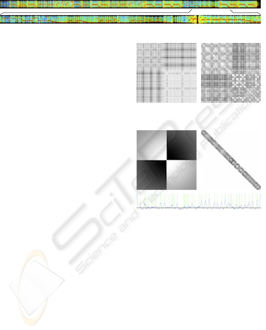
Figure 5: Zoom in a 30 seconds long portion of the song Three, by Britney Spears. Visible peaks correspond to beat onsets.

Despite being an indirect measure, the rough number

of segments that can be seen in the visual represen-

tation of an audio ﬁle leads to a reasonable evalua-

tion method, especially when the task is editing au-

dio or video, where ﬁnding separation points between

regions with distinct musical content is of great im-

portance. We have conducted an experiment to that

end, where ﬁve viewers were asked to perform the

segmentation.

Furthermore, we implemented an automatic algo-

rithm to evaluate the importance of including melodic

features in audio visualization systems. The auto-

matic procedure consists in counting the approximate

number of visible segmentation points in an audio

ﬁle when it is represented via two distinct audio fea-

tures: the loudness and the chroma vector. Since

the loudness feature represent the energy envelope of

the song, which is roughly the visible shape of the

PCM representation, this strategy allows a quantita-

tive measurement of the chroma vector importance in

audio information visualization.

We found such method of ﬁnding segmentation

points in the literature of audio summarization. It is

based in what is called the novelty score of the audio

data (Cooper and Foote, 2003).

The novelty score is deﬁned upon a structure

known as self-similarity matrix (SSM) (Foote, 1999).

Supposing we have a time-indexed array of audio fea-

tures, say v

,...,v

, the self-similarity matrix of the

audio relatively to this feature is the n × n matrix S

such that S

i, j

is s(v

), where s is some similar-

ity measure. In this work we have used s(v

) =

1 − kv

− v

k/M, where M = max

k,l

− v

Figure 6 shows and example, where an important

property of this kind of matrices can be seen: the

checkerboard pattern.

In fact the novelty score takes advantage of this

property. The idea is that convolving the main diago-

nal of such a matrix with a checkerboard kernel will

result in a curve with peaks corresponding to segment

boundaries in the song, with respect to the feature

used to build the SSM. The checkerboard kernel is de-

ﬁned as f ·g, where f (x) = +1 for x in even quadrants

and f (x) = −1 otherwise; and g(x) = e

−kxk

. Figure

7 shows the appearance of the kernel, as well as illus-

trates the process of computing the novelty score and

the novelty score itself for the chroma-SSM shown in

Figure 6.

Figure 6: Loudness (left) and chroma self-similarity matri-

ces of an about one minute long excerpt of the song Shadow

of the Day, by Linking Park.

Figure 7: Checkerboard kernel (top left) and novelty score

computation process (top right) with the corresponding re-

sulting curve (bottom) where peaks above certain threshold

are highlighted.

We have used a kernel of width 64. Consider-

ing that the audio features are computed each 2048

frames, this corresponds to about 3 seconds of audio,

which means that transitions between music parts (re-

garding the chosen audio feature) happening in such

an interval of time will be captured. The resulting

curve is smoothed to eliminate high-frequency noise,

and then normalized to the range [0, 1]. Peaks above

some threshold (0.1 for the examples presented here)

are considered to be good segmentation points.

Figure 8 shows an example of what is obtained in

our evaluation method, for the song Fireﬂies, by Owl

City. Note that in our method the rough shape of the

PCM representation is kept, and more possible seg-

mentation points are provided by the color differences

between chroma vectors.

IVAPP 2010 - International Conference on Information Visualization Theory and Applications

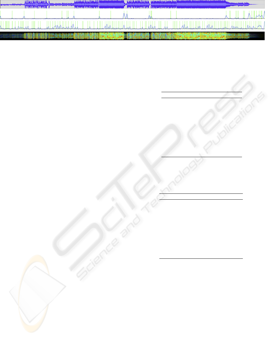
Figure 8: From top to bottom: PCM representation, loudness-based novelty score, chroma-based novelty score and our

proposed audio visualization picture.

5 RESULTS

To evaluate the importance of including melodic in-

formation when visualizing audio data for edition pur-

poses (where hints about segmentation points are de-

sirable), we have counted, for each test song, the

number of novelty score signiﬁcant peaks for the

loudness- and chroma-SSM, according to the method

described in the previous section.

As song database we chose to take the top 10 most

popular songs for the month October of 2009, accord-

ing to the website top10songs.com. Results are shown

in Table 1. Note that in all of the songs there are more

chroma peaks than loudness peaks. In fact the aver-

age ratio between the number of chroma and loudness

peaks is about 3.4.

The same songs were presented to ﬁve viewers,

who were asked to segment them using, ﬁrst, the

waveform representation, and then the representation

described in Section 3 (see Figure 9). Table 2 shows

the obtained results. Note that, except for the song

Down, the number of segments found using the wave-

form representation is always smaller. In fact the av-

erage quotient between the values in the column SP

and WF is about 1.34.

The mentioned database was also used to measure

the computational cost of the algorithm. We have

seen that the total time spent to decompress a mp3

ﬁle, compute the representation and show the result is

about 1.01 seconds per minute of audio. Regardless

of the time spent for decompressing the ﬁle, the algo-

rithm takes about 0.39 seconds per minute of audio to

execute. We have used a Macintosh machine, with a

2GHz Intel Core 2 Duo processor and 2GB of RAM,

running Mac OS X Version 10.6.2 (64-bits).

6 CONCLUSIONS

In this work we have proposed a new method for vi-

sualizing audio data for edition purposes, which is an

alternative to the ubiquitous PCM representation.

Our method is of fast computation, and is based

on the loudness and chroma audio features. By using

Table 1: Number of loudness (LP) and chroma (CP) peaks

of the novelty score using the corresponding SSM, for songs

in the testing database.

Song LP CP

I Gotta Feeling 45 71

Down 24 86

Fireﬂies 35 140

Watcha Say 48 150

Paparazzi 36 73

Party in the U.S.A. 18 134

Three 30 103

You Belong With Me 52 98

Meet Me Halfway 62 119

Bad Romance 37 183

Table 2: Average number of segments found by ﬁve view-

ers when presented to the waveform (WF) and the song pic-

ture (SP) as described in section 3, for songs in the testing

database.

Song WF SP

I Gotta Feeling 7.2 7.4

Down 7.6 6.4

Fireﬂies 9.4 9.6

Watcha Say 7.4 9.6

Paparazzi 5.8 8.4

Party in the U.S.A. 7.6 9.8

Three 6.6 13.6

You Belong With Me 4.4 9.2

Meet Me Halfway 7.8 9.8

Bad Romance 9.0 9.2

loudness, the representation resembles the traditional

PCM curve shape. The presence of chroma informa-

tion adds more hints about good segmentation points,

and can even highlight parts of the music piece that

are similar each other.

We have measured the importance of adding

melodic information (the chroma vector) in audio

visualizers by counting the number of signiﬁcative

peaks in the novelty score corresponding the chroma-

SSM for 10 different songs, and comparing with the

results corresponding to the use of the loudness-SSM.

The result is that the average ratio between the num-

ber of chroma and loudness peaks is about 3.4.

Also, ﬁve viewers were asked to segment those

songs using the PCM representation and our proposed

visualization method. In average, using our method

THE SONG PICTURE - On Musical Information Visualization for Audio and Video Editing

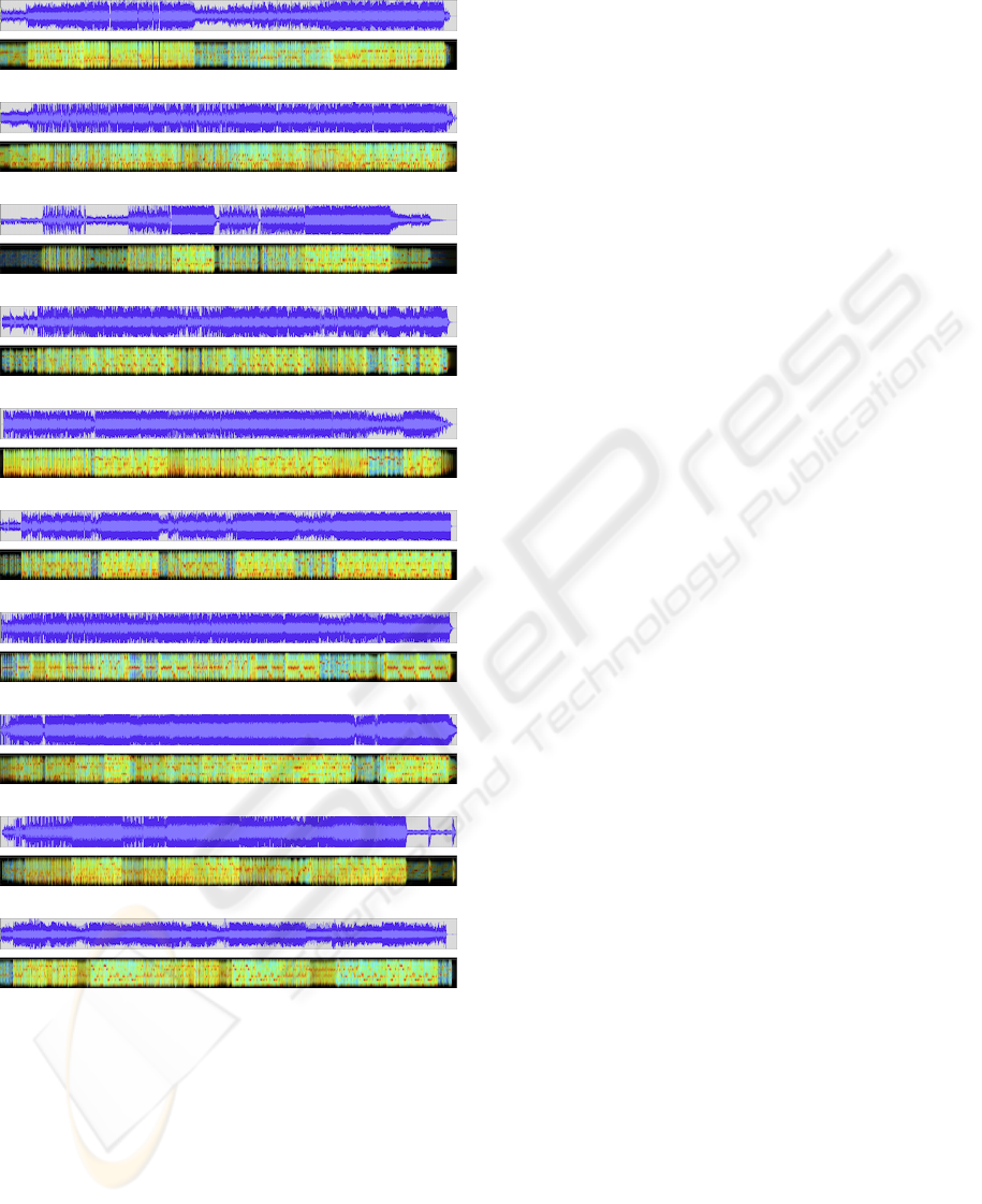
I Gotta Feeling (Black Eyed Peas)

Down (Jay Sean Featuring Lil Wayne)

Fireﬂies (Owl City)

Whatcha Say (Jason Derulo)

Paparazzi (Lady GaGa)

Party in the USA (Miley Cyrus)

Three (Britney Spears)

You Belong With Me (Taylor Swift)

Meet Me Halfway (Black Eyed Peas)

Bad Romance (Lady GaGa)

Figure 9: Song database used for the evaluation of the

method.

the number of segments found is about 1.34 times the

number of segments found when using the PCM rep-

resentation.

We believe an audio visualization method includ-

ing melodic information, like the one presented here,

could speed up the task of audio and video editing,

since the user would have more hints about bound-

aries of segments with different musical content.

The reader can test the proposed visu-

alization method by downloading the soft-

ware we have developed for this project at

www.impa.br/∼cicconet/thesis/songpicture.

REFERENCES

Azar, J., Saleh, H., and Al-Alaoui, M. (2007). Sound visual-

ization for the hearing impaired. International Journal

of Emerging Technologies in Learning.

Cicconet, M. and Carvalho, P. (2009). Eigensound: Song

visualization for edition purposes. In Sibgrapi 2009,

22nd Brazilian Symposium on Computer Graphics

and Image Processing - Poster Section.

Cooper, M. and Foote, J. (2003). Summarizing popular

music via structural similarity analysis. In Workshop

on Applications of Signal Processing to Audio and

Acoustics.

Ferguson, S., Moere, A., and Cabrera, D. (2005). Seeing

sound : Real-time sound visualisation in visual feed-

back loops used for training musicians. In Ninth In-

ternational Conference on Information Visualisation.

Foote, J. (1999). Visualizing music and audio using self-

similarity. In 7th ACM international conference on

Multimedia.

Jehan, T. (2005). Creating Music by Listening. PhD thesis,

Massachusetts Institute of Technology.

Kolhoff, P., Preuss, J., and Loviscash, J. (2006). Music

icons: Procedural glyphs for audio ﬁles. In Sibgrapi

2006, 19st Brazilian Symposium on Computer Graph-

ics and Image Processing.

Lee, M., Dolson, J., and Trivi, J. (2007). Automated visu-

alization for enhanced music playback. United States

Patent Application Publication.

Sedes, A., Courribet, B., and Thibaut, J. (2004). Visualiza-

tion of sound as a control interface. In 7th Interna-

cional Conference on Digital Audio Effects.

Verbeeck, M. and Solum, H. (2009). Method for visualizing

audio data. United States Patent Application Publica-

tion.

Ware, C. (2004). Information Visualization: Perception for

Design. Morgan Kaufmann.

IVAPP 2010 - International Conference on Information Visualization Theory and Applications