BACKGROUND MODELING WITH MOTION CRITERION AND

MULTI-MODAL SUPPORT

Juan Rosell-Ortega

Instituto de Autom´atica e Inform´atica Industrial, Universidad Polit´ecnica de Valencia, Valencia, Spain

Gabriela Andreu-Garc´ıa, Fernando L´opez-Garc´ıa, Vicente Atienza-Vanacloig

Departamento de Inform´atica de Sistemas y Computadores, Universidad Polit´ecnica de Valencia, Valencia, Spain

Keywords:

Background subtraction, Surveillance, Motion segmentation.

Abstract:

In this paper we introduce an algorithm aimed to create a background model with multimodal support, which

associates a conﬁdence value to the obtained model. Our algorithm creates the model based on a criterion of

motion, pixel behavior and pixel similarity with the scenes background. This method uses only three frames

to create a ﬁrst model without restrictions on the frame content. The model is adapted over time to reﬂect new

situations and illumination changes in the scene. One approach to detect corrupt model is also mentioned.

The goal of conﬁdence value is to quantify the quality of the model after a number of frames have been used

to build it. Quantitative experimental results are obtained with a well-known benchmark and compared to a

classical background modelling algorithm, showing the beneﬁts of our approach.

1 INTRODUCTION

Background subtraction is one of the most popu-

lar methods to detect regions of interest in frames.

This technique consists in classifying as foreground

all those pixels whose difference from a background

model is over a threshold. A popular method for back-

ground modelling consists in modelling each pixel

in a frame with a Gaussian distribution (Wren et al.,

1997). A simple technique is to calculate an aver-

age image of the scene, to subtract each new video

frame from it and to threshold the result. The adap-

tive version of this algorithm updates the model pa-

rameters recursively by using a simple adaptive ﬁlter.

The Gaussian distribution approach however,does not

work well when the background is not static, for in-

stance, waves, clouds or any movement which also

belongs to the background cannot be properly de-

scribed using one Gaussian. A solution proposed

(Stauffer and Grimson, 1999) is using more than one

Gaussian to model the background. In (Zang and

Klette, 2004) methods for shadow detection and per-

This work has been supported partially by the research

projects DPI2007-511 66596-C02-01 (VISTAC) and Euro-

pean SENSE Project 033279

pixel adaptation of the parameters of the Gaussians

are developed. Following with the methods based on

mixture of Gaussians, in (Elgammal et al., 2000), it

is proposed to build an statistical representation of

the background, by estimating directly from data the

probability density function. Other approaches can

be found in (Mason and Duric, 2001), whose pro-

posed algorithm computes a histogram of edges in a

block basis. This idea together with intensity infor-

mation may be found in (Jabri et al., 2000). Mo-

tion may also be used to model the background as

proposed in (Wixson, 2000), whose algorithm detects

salient motion by integrating frame-to-frame optical

ﬂow over time. Radically different is the approach

based in LBP features introduced in(M. Heikkila and

Pietikainen, 2006). In general, the use of frames with

low or very low activity is one of the constraints con-

sidered in these approaches.

We focus on demanding scenarios, in which there

is always a signiﬁcant activity level, making it dif-

ﬁcult to obtain a clean model with traditional tech-

niques. Our method aims to obtain a model regardless

of the number of objects moving in the scenario while

building the model. A quality measure is developed

with the aim of measuring the quality of the obtained

model.

419

Rosell-Ortega J., Andreu-García G., López-García F. and Atienza-Vanacloig V. (2010).

BACKGROUND MODELING WITH MOTION CRITERION AND MULTI-MODAL SUPPORT.

In Proceedings of the International Conference on Computer Vision Theory and Applications, pages 419-422

DOI: 10.5220/0002822604190422

 SciTePress

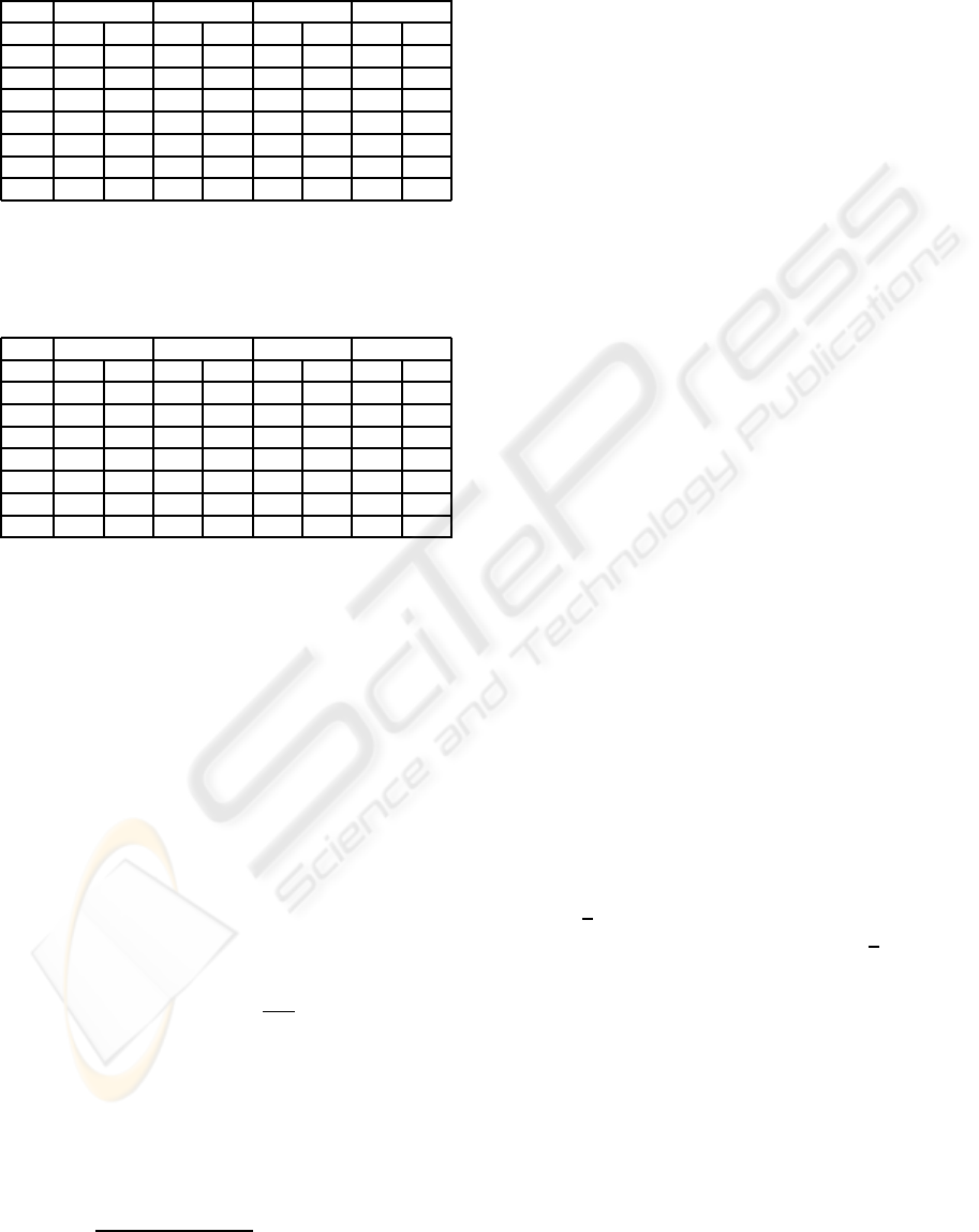
Table 1: Results obtained for the Wallﬂower benchmark us-

ing equation 5 to detect foreground regions with γ = 0.6.

Dashed results mean that no foreground pixels were labelled

in the control image.

κ = 5 κ = 10 κ = 15 κ = 20

Seq. TP TN TP TN TP TN TP TN

boo. 0.67 0.82 0.55 0.93 0.48 0.96 0.41 0.97

cam. 0.40 0.89 0.15 0.95 0.72 0.91 0.70 0.92

fore. 0.72 0.30 0.53 0.80 0.49 0.90 0.47 0.99

lig. 0.43 0.98 0.33 0.97 0.26 0.98 0.21 0.98

mov. - 1 - 1 - 1 - 1

tim. 0.70 0.95 0.48 0.97 0.37 0.98 0.31 0.98

wav. 0.91 0.56 0.86 0.68 0.80 0.76 0.74 0.80

Table 2: Results obtained for the Wallﬂower benchmark us-

ing equation 5 to detect foreground regions with γ = 0.4.

Dashed results mean that no foreground pixels were labelled

in the control image.

κ = 5 κ = 10 κ = 15 κ = 20

Seq. TP TN TP TN TP TN TP TN

boo. 0.87 0.43 0.59 0.92 0.55 0.94 0.50 0.95

cam. 0.74 0.74 0.77 0.90 0.72 0.90 0.70 0.93

fore. 0.90 0.60 0.49 0.98 0.24 0.99 0.20 0.99

lig. 0.82 0.15 0.30 0.86 0.48 0.90 0.47 0.91

mov. - 0.97 - 1 - 1 - 1

tim. 0.83 0.77 0.42 0.98 0.35 0.98 0.30 0.98

wav. 0.96 0.32 0.86 0.67 0.81 0.73 0.75 0.79

2 MULTI-MODAL BACKGROUND

ADAPTIVE WITH

CONFIDENCE ALGORITHM

(MBAC)

MBAC considers consecutive gray scale frames

F(0),F(1), ...F(n), in which any pixel p ∈ F(i) be-

longs either to foreground or to background and

builds a background model B starting from a frame

F(i),i ≥ 0, by describing each pixel b with a num-

ber of models B

(0), with m = 1 at t = 0. Pixels are

classiﬁed following the similarity criterion proposed

in (Rosell-Ortega et al., 2008). This criterion uses a

continuous function deﬁned as,

S(p,b) = e

−

|p−b|

(1)

being p the gray level of a pixel and b the gray

level of a background pixel, and κ a constant. Motion

can be computed analogously if we consider motion

as the dissimilarity with values of previous frames.

For q ∈ F(t) a pixel in the current frame, we consider

p ∈ F(t − 1) and r ∈ F(t − 2), two pixels with the

same coordinates as q, the motion of q can be deﬁned

as M(q) =

(1−S(p,q))+(1−S(r,q))

MBAC starts setting ∀b ∈ B,1 ≤ m ≤ K(b) :

(0) = F

(i),c

(0) = 0.01, being c

(0) the conﬁ-

dence value of the m-th model of pixel b in time i = 0.

This conﬁdence value measures how good the model

describes the pixel. The parameter K(b) limits the

maximum number of models for pixel b. Initially,

only one model per pixel is considered. The follow-

ing two frames, F(i + 1) and F(i + 2), are ignored

and used only to detect motion in frame F(i+ 3). For

all the following frames F( j), j ≥ i + 3, motion and

similarities with B(i− 1) are seeked. The probability

that any pixel q belongs to background pBack(q) or

foreground, pFore(q) is,

pBack(q) = max(1− M(q),max(S(q,B

)))) (2)

pFore(q) = max(M(q),1− max(S(q,B

))) (3)

It is easy to see, that equation for pBack(q) de-

scribes mathematically the intuitive idea that pixels

similar to background or which are reasonably sta-

tionary have a bigger probability of belonging to

background. The segmentation separates pixels in

two different sets; the background set (bSet), deﬁned

as bSet = {p ∈ F(i) : p /∈ fSet}, and the foreground

set (fSet).

fSet = {p ∈ F(i) : pFore(p) > τ} (4)

In the previous expression for fSet, the value of τ

restricts the criteria used to select foreground pixels.

This expression can be rewritten as,

fSet = {p ∈ F(i) : pFore(p) > pBack(p)} (5)

After classifying pixels, a simple criterion to de-

tect corrupt models is used. We assume that the

amount of background pixels (V) is bigger than that

of foreground pixels (P). If R = P+V, a real number

µ < 1 can be found that P = µ × R. The value µ is set

experimentally depending on background clutter. In

the case

> µ at time i, the process restarts setting

∀b ∈ B,B

(0) = F

(i), c

= max(c

). If

≤ µ, the

model is updated with information of frame F(i) In

order to cope with light changes. The model m which

matched the background for a pixel b is updated as,

(i) = α B

(i− 1) + (1− α) F

(i) (6)

(i) = α c

(i− 1) + (1− α) pBack(b) (7)

Any other non-matching model l describing pixel

b updates its conﬁdence as,

(i) = α c

(i− 1), ∀l 6= m (8)

VISAPP 2010 - International Conference on Computer Vision Theory and Applications

420

Table 3: The two columns on the left show true posi-

tives and negatives percentages of algorithm MBAC for the

Wallﬂower benchmark. On the right, results for the Stauffer

algorithm.

MBAC Stauffer BAC

TP TN TP TN TP TN

bootstrap 0.52 0.94 0.44 0.97 0.60 0.91

camouﬂage 0.73 0.90 0.73 0.92 0.75 0.76

foregroundAperture 0.48 0.92 0.50 0.85 0.48 0.90

lightSwitch 0.24 0.97 0.73 0.07 0.28 0.98

movedObject - 1.00 - 1.00 - 1.00

timeOfDay 0.36 0.97 0.41 0.98 0.36 0.98

wavingTree 0.75 0.75 0.86 0.90 0.78 0.67

where α ∈ [0,1] is a learning rate factor. For every

pixel p ∈ fSet, its m background models are ordered

in descending order according to their conﬁdences.

We use a parameter gamma to control the speed at

which models are changed or updated in the back-

ground model. The closer gamma is to 1, the quicker

models will be added or updated. In the case it is

veriﬁed that s = Σc

(i),1 ≤ m ≤ K(p) < γ , a new

model will be added or the worst model will be re-

placed. For the new model m, the algorithm sets

(i) = F(i),c

(i) = 0.01.

3 EXPERIMENTS AND RESULTS

We used the Wallﬂower benchmark (Toyama et al.,

1999) in order to compare our approach to Stauffer’s

algorithm (Stauffer and Grimson, 1999) and BAC

(Rosell-Ortega et al., 2008). We compared the num-

ber of pixels classiﬁed as foreground and labelled as

foreground in the control image (true positives) and

those pixels classiﬁed as background and also classi-

ﬁed as background in the control image (true nega-

tives).

We used K = 5 and T = 0.8 as parameters for the

Stauffer algorithm. Parameters for MBAC were set

after a previous study of their impact in the execution.

Tables 2 and 1 show the results obtained by varying

the values of κ in equation 1 and its impact depending

on the value of γ used. Results seem to be better with

a low γ. Tables 4 and 5 show the results of using each

deﬁnition of pFore in equation 4. As a conclusion

of these experiments, the segmentation seems to im-

prove slightly when a strict value for τ is chosen. The

remaining parameters of MBAC are κ = 20, µ = 0.85,

γ = 0.4 and τ = 0.8.

Table 3 illustrates the results with the Wallﬂower

benchmark. Qualitative results are shown in ﬁgure

1. In sequence lightSwitch, MBAC manages prop-

erly the sudden light change restarting the model,

while Stauffer’s algorithm fails to deal with the sit-

uation. The most signiﬁcant improvement of MBAC

over BAC, is achieved in sequences wavingTrees and

camouﬂage. In all cases MBAC achieved over 80%

of success in the classiﬁcation of background pixels.

4 CONCLUSIONS AND FUTURE

WORKS

We introduced an approach in which similarity and

motion features are used to classify pixels as fore-

ground or background. Considering motion at the

same level as background subtraction with several

models produces accurate background models but at

the expense or reducing the amount of regions of in-

terest detected if thresholds are not accurate enough.

This issue remains as an open line for further re-

search.

REFERENCES

Elgammal, A., Harwood, D., and Davis, L. (2000).

Non-parametric model for background subtraction.

ECCV00, pages 751 767.

Jabri, S., Duric, Z.,Wechsler, H., and Rosenfeld, A. (2000).

Detection and location of people in video images un-

sing adaptive fusion of color and edge information.

IEEE Proc. ICPR00, pages 627 630.

M. Heikkila, M. and Pietikainen, M. (2006). A texture-

based method for modeling the background and

detecting moving 0bjects. IEEE Trans. PAMI,

28(4):657662.

Mason, M. and Duric, Z. (2001). Using histograms to detect

and track objects in color video. Proc. Applied Imag-

inery pattern Recognition Workshop, pages 154159.

Rosell-Ortega, J., Andreu-Garcia, G., Rodas-Jorda, A.,

and Atienza-Vanacloig, V. (2008). Background mod-

elling in demanding situations with conﬁdence mea-

sure. IEEE Proc. ICPR08.

Stauffer, C. and Grimson, W. E. L. (1999). Adaptive back-

ground mixture models for real-time tracking. Proc.

IEEE CVPR99, pages 246 252.

Toyama, K., Krumm, J., Brumitt, B., and Meyers, B.

(1999). Wallﬂower: Principles and practice of back-

ground maintenance. IEEE ICPR99, Kerkyra, Greece,

pages 255261.

Wixson, L. (2000). Detecting salient motion by accumulat-

ing directionally-consistent ﬂow. IEEE Trans. PAMI,

8(22):774 780.

Wren, C. R., A. Azarbayenjani, T. D., and Pentland, A. P.

(1997). Pﬁnder: rel-time tracking of the human body.

IEEE Trans. PAMI, 10(7):780 785.

Zang, Q. and Klette, R. (2004). Robust background subtrac-

tion and maintenance. IEEE ICPR04, pages 90 93.

BACKGROUND MODELING WITH MOTION CRITERION AND MULTI-MODAL SUPPORT

421

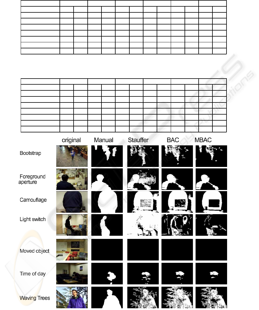
Table 4: Results obtained for the Wallﬂower benchmark depending on the value assigned to the minimum foreground proba-

bility with γ = 0.6. Dashed results mean that no foreground pixels were labelled in the control image.

τ = 0.4 τ = 0.5 τ = 0.6 τ = 0.7 τ = 0.8 τ = 0.9

Sequence TP TN TP TN TP TN TP TN TP TN TP TN

bootstrap 0.62 0.89 0.59 0.91 0.54 0.92 0.48 0.96 0.39 0.97 0.30 0.99

camouﬂage 0.13 0.95 0.73 0.86 0.73 0.90 0.70 0.91 0.72 0.93 0.69 0.94

foregroundAperture 0.49 0.88 0.48 0.90 0.48 0.90 0.47 0.92 0.47 0.93 0.46 0.93

lightSwitch 0.44 0.97 0.36 0.97 0.27 0.97 0.20 0.99 0.63 0.17 0.55 0.22

movedObject - 1 - 1 - 1 - 1 - 1 - 1

timeOfDay 0.51 0.95 0.43 0.96 0.32 0.98 0.30 0.98 0.28 0.98 0.26 0.98

wavingTree 0.94 0.50 0.88 0.59 0.79 0.73 0.69 0.79 0.58 0.86 0.46 0.92

Table 5: Results obtained for the Wallﬂower benchmark depending on the value assigned to the minimum foreground proba-

bility. The value of γ was set to 0.4. Dashed results mean that no foreground pixels were labelled in the control image.

τ = 0.4 τ = 0.5 τ = 0.6 τ = 0.7 τ = 0.8 τ = 0.9

Sequence TP TN TP TN TP TN TP TN TP TN TP TN

bootstrap 0.71 0.79 0.67 0.83 0.61 0.88 0.58 0.91 0.52 0.94 0.44 0.97

camouﬂage 0.45 0.92 0.34 0.92 0.79 0.78 0.75 0.86 0.73 0.90 0.71 0.91

foregroundAperture 0.69 0.53 0.62 0.71 0.51 0.88 0.48 0.90 0.48 0.92 0.47 0.93

lightSwitch 0.53 0.95 0.44 0.96 0.36 0.98 0.29 0.93 0.24 0.97 0.18 0.99

movedObject - 1 - 1 - 1 - 1 - 1 - 1

timeOfDay 0.74 0.93 0.66 0.94 0.52 0.97 0.44 0.97 0.36 0.97 0.30 0.98

wavingTree 0.98 0.41 0.94 0.47 0.90 0.59 0.83 0.67 0.75 0.75 0.65 0.82

Figure 1: Detection results per sequence. Column on the left corresponds to the control frame segmented by hand, central

column shows the result obtained by BAC and column on the right represents results obtained by MBAC.

VISAPP 2010 - International Conference on Computer Vision Theory and Applications

422