THE STRUCTURAL FORM IN IMAGE CATEGORIZATION

Juha Hanni, Esa Rahtu and Janne Heikkil

Machine Vision Group, Department of Electrical and Information Engineering, University of Oulu, Finland

Keywords:

Image categorization, Clustering, Generative model.

Abstract:

In this paper we show an unsupervised approach how to ﬁnd the most natural organization of images. Previous

methods which have been proposed to discover the underlying categories or topics of visual objects create no

structure or at least the structure, usually tree-shaped, is deﬁned in advance. This causes a problem since the

most relevant structure of the data is not always known. It is worthwhile to consider a generic way to ﬁnd

the most suitable structure of images. For this, we apply the model of ﬁnding the structural form (among

eight natural forms) to automatically discover the best organization of objects in visual domain. The model

simultaneously ﬁnds the structural form and an instance of that form that best explains the data. In addition, we

present a generic structural form, so called meta structure, which can result in even more natural connections

between clusters of images. We show that the categorization results are competitive with the state-of-the-art

methods while giving more generic insight to the connections between different categories.

1 INTRODUCTION

As more and more images and image categories

become available, organizing them is crucial. By

learned organization we can enable a quicker iden-

tiﬁcation of an unknown object, explore the relations

between the clusters of images and easily ﬁnd cate-

gories similar to each other. This can help us to obtain

a better classiﬁcation result.

Recent applications considering previous issues

are presented at least in (Sivic et al., 2008; Bart et al.,

2008; Marszalek and Schmid, 2008). Relations be-

tween categories can also be useful in object recog-

nition and detection, as shown in (Ahuja and Todor-

ovic, 2007; Parikh and Chen, 2007). A drawback here

is that all the previous methods deal with tree-shaped

structures only.

Unsupervised probabilistic latent topic discovery

models like probabilistic Latent Semantic Analysis

(pLSA) and Latent Dirichlet Allocation (LDA), ear-

lier used in text categorization (Blei et al., 2003; Hoff-

mann, 2001), are straightforward to employ in case of

visual data by using visual vocabulary (Sivic et al.,

2005; Bosch et al., 2006). These models create a ﬂat

topic structure where each document has a probabil-

ity of belonging to each topic. To extract the relations

between topics, a hierarchical LDA has recently been

applied to image data in (Sivic et al., 2008). They

showed it to improve the classiﬁcation accuracy but

this method exploits again only a tree-shaped struc-

ture to describe the relations between topics. A better

way still might be to look more inside the data and

ﬁnd the structure that best describes it. This way we

can exploit the gained organization most.

In this paper, we simultaneously categorize im-

ages and ﬁnd the best structure to describe the con-

nections between categories, all in an unsupervised

manner. In other words, we propose a method which

gives us a chance to learn automatically the most nat-

ural structure of images instead of using a ﬁxed struc-

ture. The method we use is based on the algorithm

introduced in (Kemp and Tenenbaum, 2008).

We improve the algorithm to consider also a so

called meta structure. In theory, a meta structure can

adapt to any structure that exists. In addition, we pro-

pose how to add samples to a given structure and how

this algorithm can be applied to large datasets. The

experiments reveal a competitive classiﬁcation accu-

racy, and furthermore, the generated structures ﬁt the

data seemingly well.

This paper is organized as follows. Section 2 re-

views shortly the algorithm of discovering the struc-

tural form and shows the improvements we made. In

section 3, we show how to employ this method in vi-

sual domain. Section 4 then describes the experiments

made on two set of images: MSRC-B1 dataset and a

345

Hanni J., Rahtu E. and Heikkilä J. (2010).

THE STRUCTURAL FORM IN IMAGE CATEGORIZATION.

In Proceedings of the International Conference on Computer Vision Theory and Applications, pages 345-350

DOI: 10.5220/0002821403450350

 SciTePress

set of faces. Finally, section 5 presents our conclu-

sions.

2 THE STRUCTURAL FORM

In this section, we ﬁrst shortly review the basics of

the algorithm of discovering the structural form. This

algorithm tries to ﬁnd a structure (among eight natu-

ral forms) which describes the data most likely. The

structures are presented by graphs and each graph is

characterised by a speciﬁc graph grammar. The nodes

of the graph represent categories and the edges repre-

sent similarities between the categories. A grammar

deﬁnes now a generative process to create a structure.

Note that each form has its own speciﬁc grammar

which can be described as a node splitting rule for

the generative process.

To go further on this subject, we prefer to have

a more ﬂexible structure to describe the relations be-

tween categories than any of the used forms. Thus

the end of this section concentrates on how to make

it possible to learn an instance of a meta structure by

using a meta-grammar which consists of several node

splitting rules.

2.1 Discovering the Structural Form

The approach described here is adapted from (Kemp

and Tenenbaum, 2008) (matlab implementation avail-

able online) and we call it ”Kemp’s algorithm” or just

”the algorithm”.

We deﬁne form F to be any of the following

forms: partition, chain, order, ring, hierarchy, tree,

grid and cylinder. Structure S, generated from form

F, is presented by a graph with nodes corresponding

to clusters of entities. An entity graph, S

ent

, is a graph

where entities are included to cluster nodes by adding

an extra node for each entity and connecting it by an

edge to the cluster node which entity is assigned to.

An example is presented in ﬁgure 1.

Let D be an n × m entity-feature matrix and S a

structure of form F. We are now searching for a struc-

ture and form which together maximize the posterior

probability

P(S,F|D) ∝ P(D|S)P(S|F)P(F), (1)

where P(F) is a uniform distribution over all the pos-

sible forms considered.

Probability P(S|F) in equation (1) is the proba-

bility of that the structure is generated from a given

form. We deﬁne

P(S|F) ∝



|S|

, if S is compatible with F

0, otherwise,

(2)

Figure 1: (A) Eight structural forms. (B) A structure on

the left is compatible with grid structure while the other one

is not. (C) The entity graph obtained from the left one in

spot(B).

where |S| is the number of nodes in graph S and

θ ∈ (0,1). Structure S is compatible with form F if it

can be generated using the generative process (graph

grammar) deﬁned for F and if graph does not contain

empty nodes when projected along its component di-

mensions. The latter notion is relevant in the case of

grids and cylinders to prevent them from getting too

complex, meaning many empty nodes in the graph.

Probability P(S|F) is deﬁned so that if the num-

ber of nodes in graph is large, it gives smaller values

(bigger penalty for the model). Let |S| be the number

of nodes in graph S. When we write θ = exp(−x),

x > 0, log likelihood log P(S|F) = |S|log(θ) = −|S|x

decreases by a constant x whenever an additional node

is introduced. This way we tend to get small and sim-

ple graphs when using bigger values of x.

Secondly, we want to ﬁnd a structure of a given

form that ﬁts best the data. This is achieved by maxi-

mizing the probability P(D|S) = P(D|S

ent

) by assum-

ing that feature values in data matrix D are indepen-

dently generated from a multivariate Gaussian distri-

bution with dimension for each node in the graph S

ent

This means that P(D|S) is high if the features in ma-

trix D vary smoothly over the graph S, that is, if enti-

ties nearby in S have similar feature values.

Let W = [w

i j

] be a weight matrix, i.e. a matrix

which is comparable with edge lengths in entity graph

ent

. We deﬁne w

i j

whenever nodes i and j are

connected by an edge with length of e

i j

, otherwise w

i j

= 0. A generative model for a single feature vector f

that favours now the feature values f

to be similar in

nearby nodes in S

ent

is given by

P( f |W ) ∝ exp(−

∑

i, j

i j

( f

− f

)

) = exp(−

∆ f ),

VISAPP 2010 - International Conference on Computer Vision Theory and Applications

346

where ∆ = E −W , is the graph Laplacian and E is a

diagonal matrix e

∑

i j

Finally, by assuming that a feature value f

at any

entity node has an a priori variance of σ

, we obtain

a proper priori f |W ∼ N(0,

∆

−1

), where

∆ is ∆ with

1/σ

added on the diagonal of the ﬁrst n positions.

Note that the entity graph S

ent

and weight matrix W

are deﬁned so that the entities are in the ﬁrst n posi-

tions and the rest are the latent cluster nodes.

The priors for edge lengths e

i j

and for σ are drawn

from exponential distribution with parameter β = 0.4,

as in (Kemp and Tenenbaum, 2008). Now we can

compute the likelihood P(D|S

ent

,W,σ) and

logP(D|S

ent

,W,σ) = log

∏

i=1

P( f

|W ) =

log(2π) −

log|

∆

−1

| −

tr(

∆DD

(3)

where m is the number of feature vectors and f

the ith feature vector. By integrating out σ and edge

weights we obtain the likelihood P(D|S

ent

For further information, we refer on (Kemp and

Tenenbaum, 2008).

2.2 Assigning New Data to a Learned

Structure

It is interesting to notice that the algorithm does not

necessarily need the feature data D itself but can use a

covariance matrix

. As long as we know this

covariance matrix, this approach can be used even

though we actually do not have the actual features.

This means that we can learn structures from some

similarity matrix by assuming that this similarity ma-

trix represents a covariance matrix of the data. We

prefer to use similarity matrix due to its ability of be-

ing ﬂexible to choose. If the metric of a feature space

cannot reveal the relations between observations, it is

worth using a suitable similarity measure. Later on,

we run into previous matter in case of histogram data.

For classiﬁcation purposes it would be convenient

to be able to add new samples to a given structure. To

assign a new sample, ﬁrst we compute the similarities

of the sample and the training samples used to build

the structure. One by one, we go through all the clus-

ter nodes and join the new sample by an edge to the

node we are visiting to. In each case at a time, we

can compute the likelihood in equation (3). The edge

weight between the new sample and a cluster node is

set to be the mean value of all edge weights in the

graph. Although edge weights can be optimized, we

found it to be quite ineffectual and slow when deal-

ing with hundreds of samples. Finally, the sample is

assigned to the cluster node which gives the highest

Figure 2: Node splitting rules for a meta-grammar. On the

right side the correspondences with the primitive forms hav-

ing the same grammar. Note that we cannot do the very ﬁrst

split by the 4th rule, because we want graph to be connected.

likelihood score. The probability P(S|F) can obvi-

ously be forgotten since the cluster graph S is ﬁxed.

2.3 A Meta-grammar

Using the eight presented forms can still lead to the

circumstances where the structures simply cannot re-

veal the true, possibly complex, nature of the data.

This leaves a room for a more generic form. As men-

tioned earlier, each form is characterised by the gram-

mar it uses to split the nodes. When a grammar is

an arbitrary mixture of several grammars, we call it

a meta-grammar and a structure that uses this meta-

grammar is called a meta structure. The idea of a

meta-grammar was introduced in (Kemp and Tenen-

baum, 2008) but was never used. The template of that

meta-grammar was a combination of grammars of the

six forms (all but grid and cylinder), so called primi-

tive forms, illustrated in ﬁgure 1.

In this paper, we propose a slightly different meta-

grammar and also put it into practice. The choices

for node splits that our meta-grammar uses are shown

in ﬁgure 2. First, we do not allow any nodes in the

graph to be empty. For example the node splitting rule

i.e. generative process used to create trees is not valid

since the branch nodes will be empty. Secondly, we

do not want to split the graph into two disjoint graphs

so the very ﬁrst split cannot be done by the genera-

tive process designed for partition structure. These

notions allow us to make simple, connected graphs.

The two rightmost rules in ﬁgure 2 do not generate

any natural structure themselves but give a necessary

(and sufﬁcient) complement to our meta-grammar.

Using this meta-grammar provides the graph with

more opportunities to organize itself. In practise, to

split a node, we try each splitting rule present in a

meta-grammar and choose the best one with respect

to the likelihood (3).

One problem we face now is the difﬁculty of com-

puting the probability P(S|F). The normalization

constant for the distribution in (2) is the sum

∑

P(S|F) =

∑

k=1

S(n,k)C(F,k)θ

, (4)

where S(n,k) is the number of ways to partition n ele-

ments into k nonempty sets and C(F, k) is the number

THE STRUCTURAL FORM IN IMAGE CATEGORIZATION

347

of structures of form F with k occupied cluster nodes.

When considering the form of meta structure and

the number of possibilities how the meta-grammar

can generate a structure with k nodes, we can clearly

see that computing the exact number C(F,k) is too

hard. Anyway, we can easily ﬁnd a rough upper limit

for the number C(F, k), since we can easily verify that

the number of ways to draw edges in the case of k

cluster nodes is 2

k(k−1)/2

. Thus, we have a lower

boundary for likelihood P(S|F).

3 THE ORGANIZATION OF

VISUAL OBJECTS

We represent images as histograms of quantized de-

scriptors. This bag-of-words (BOW) method has

been successfully used in many papers such as (Sivic

et al., 2008; Marszalek and Schmid, 2008; Bosch

et al., 2006). Moreover, we extract descriptors from

a grayscale image by computing the SIFT-features

(Lowe, 2004) on a dense grid using an implementa-

tion available online (van de Sande et al., 2010).

As stated in section 2.2, we can use a similarity

matrix of the histograms as an input to the algorithm.

Besides, due to computational efﬁciency of the algo-

rithm, we found the similarity matrix behave better

than pure feature data. To compute the similarity ma-

trix we transform χ

-distances between histograms to

similarity values within range [0,1].

For reasonable execution time of the algorithm,

we can use only a subset of samples to ﬁnd the

best structure and assign the rest of the samples to

a learned structure, as described in section 2.2. More

speciﬁcally, the samples which have a small variance

in similarities are excluded from the training process.

Although, the algorithm decides itself which is the

best structure, we can also examine different struc-

tures manually by comparing extracted log likeli-

hoods, logP(S,F|D), of the model.

3.1 Assessing Structures using

Classiﬁcation

In evaluation, we use the same ”classiﬁcation overlap

score”, as described in (Sivic et al., 2008). Classiﬁca-

tion overlap score indicates how well the entities of a

particular, manually labeled, object class are assigned

to a single node in a tree. Obviously, we want high re-

call and high precision, so we want most of the class

attributes to have a common node, which hopefully

does not contain attributes from another class. The

scale of this score is from 0 to 1. If score is 1 then

all object classes are fully separated at some node in

the structure. Disadvantage is that this score is not di-

rectly usable in case of the other structures than tree or

partition. One possibility is to modify the structures

to be tree-shaped in a way we next describe.

As we know, the results of the algorithm are ba-

sically weighted graphs. Cluster graphs are graphs

with no separate edges between entities and cluster

nodes, as we have declared earlier. For each cluster

graph, multiple clustering is obtained by running the

Normalized Cuts (Shi and Malik, 2002) with vary-

ing the number of clusters. After this, we create a

co-occurrence matrix of how many times each pair

of the nodes in the graph appears in the same clus-

ter. This matrix can be used as a similarity matrix

for the hierarchical agglomerative clustering (Hastie

et al., 2009), which creates a tree structure. After this

operation, we are able to assess the classiﬁcation ac-

curacy based on the classiﬁcation overlap score, re-

gardless of the structure type.

It is apparent that the nature of structures suffers

from this transformation and this measure suits better

for tree-shaped structures. However, we have no other

measure on hand at the moment so we trust that this

measure gives at least a good estimate of the classiﬁ-

cation ability of each structure.

4 EXPERIMENTS

4.1 MSRC Dataset

We consider now a dataset MSRC-B1 (Winn et al.,

2005) consisting of 240 images which are manually

segmented to 12 different object classes. We use 543

segments of 9 different object classes: faces, cows,

grass, trees, buildings, cars, airplanes, bicycles and

sky. Other three classes: sheep, horses and ground

are represented by only so few samples that we ignore

them. This is exactly similar to (Sivic et al., 2008).

The SIFT-descriptors are computed at every 5th

pixel in an image. Each image segment is then de-

scribed by all visual words with centroids within the

segment. We use 150 segments as a training data for

ﬁnding the structure and assign the remainder to the

Figure 3: Log-likelihoods of each structure in case of data

MSRC-B1. A constant has been added along y-axis so that

the worst performing structure receives score close to zero.

The best performing structure is marked by an asterisk.

VISAPP 2010 - International Conference on Computer Vision Theory and Applications

348

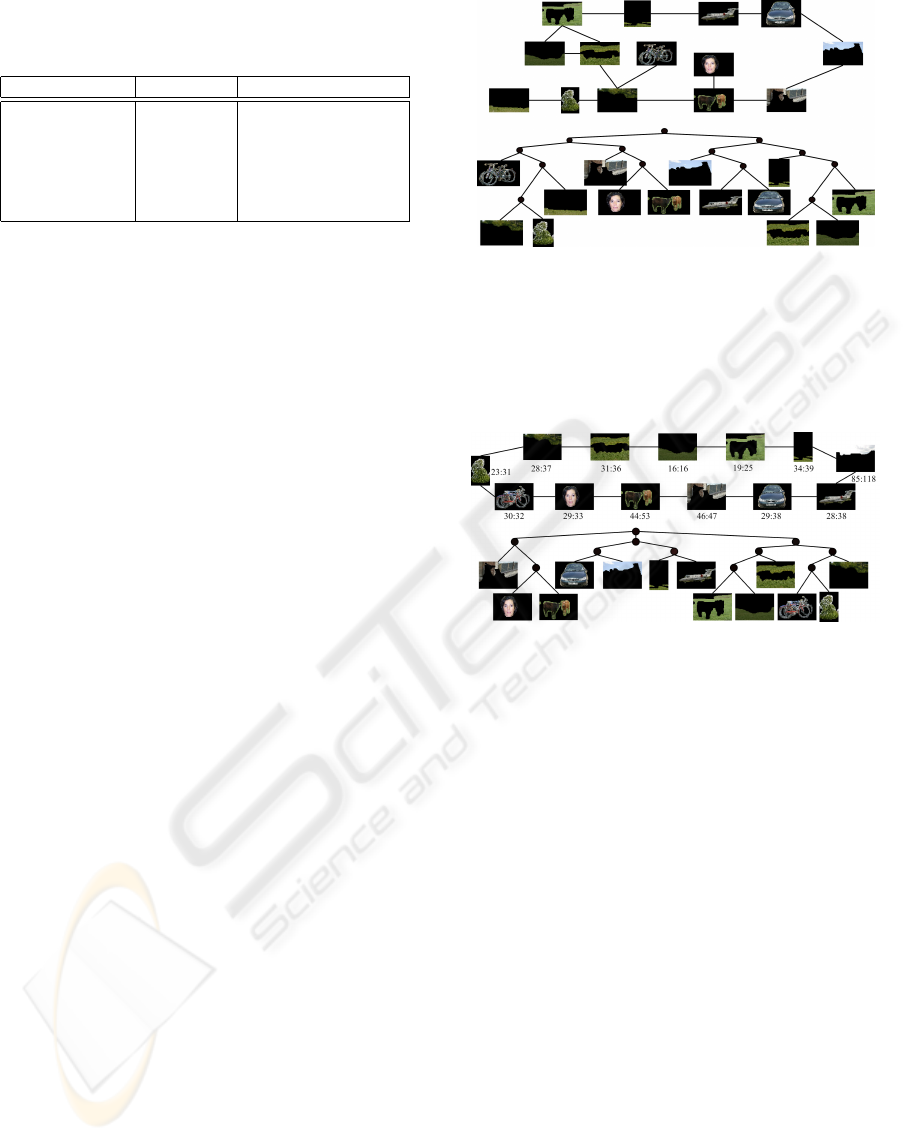
Table 1: Image classiﬁcation accuracy on MSRC-B1 data.

Accuracy is measured by classiﬁcation overlap score. The

results of our method are the average of ten repeats.

method topics score

LDA 5/10/15/20 0.50/0.46/0.57/0.61

hLDA - 0.72

partition 8 0.53

tree, ring 15 0.65

meta 16 0.65

other structures 11-15 0.44-0.63

(Sivic et al., 2008)

learned structure. We set θ = exp(−200) for all forms

considered and use a vocabulary of size one thousand

words. The vocabulary is obtained by using all the

samples.

4.1.1 Comparision of the Structures

In the case of the tree and partition structure we can

compute the classiﬁcation overlap score directly. For

other structures we use the method described in sec-

tion 3.1. The results are shown in table 1.

When compared to the results of LDA, the parti-

tion structure gives a better score with respect to the

number of clusters. It gives eight clusters which is

much closer to the number (9) of manually labeled

classes than in the case of the best score (20 clusters)

achieved by LDA. Most of the other structures give

better results when compared to the best gained by

LDA. We also see that hLDA gives better results in

this case but our results are still comparable, in spite

of forcing a tree-shape to the structures.

Figure 3 indicates how the meta structure is the

model’s choice of the best structure now. However,

when comparing the classiﬁcation accuracy, the ring,

tree and meta structures all get the same score. The

meta, ring and tree structures are presented in ﬁgures

4, 5. The clusters formed by each structure are quite

similar to each other but the relations between clus-

ters differ. It seems quite fair that meta structure wins

when looking at the graphs. Although, in this case

some of the clusters (for example buildings) are very

different from the rest and meaningful connections

are diffucult to draw even for a human.

When comparing the results with the hierarchy in

(Sivic et al., 2008), it appears that our approach cre-

ates more natural clustering than hLDA does. Unlike

in our results, the number of small, meaningless clus-

ters is large in their approach. We may say that by

making more compact categorization, we lose some

units in accuracy.

To return to the aspect of this paper, hLDA has

one disadvantage when it comes to the possible rela-

tionships which a tree structure or any other structure

Figure 4: Uppermost the meta structure learned on the

MSRC-B1 dataset of 543 image segments of 9 object

classes. The images presenting each cluster are chosen to

be the ones which are the most similar with the clusters’

majority class. The edge lengths correspond to the edge

weights. Down below a tree-shaped structure obtained from

the meta structure by combining normalized cuts and hier-

archical clustering.

Figure 5: The ring and tree structures learned on the MSRC-

B1 dataset. The images presenting each cluster are chosen

to be the ones which are the most similar with the clusters’

majority class. In the case of the ring structure, nodes are la-

beled by the number of images coming from the same class

as the representative image of the node versus the number

of all images in the node.

deﬁned in advance cannot reveal. In the previous ex-

ample, a tree-shaped structure worked as well as any

since the image categories hardly shared anything in

common. What about when the categories really have

some underlying structure. How can we be sure that

a certain chosen structure really match the data then?

That is why it is good to consider a more generic view

on creating the structure of images to gain deeper in-

sight for any use of the structure.

4.2 Face Dataset

Let us then consider a situation where we have ex-

actly one feature that is assumed to describe a set of

images. If the values of this feature varies smoothly

between images, we can imagine that it is not easy or

even possible to get this information stored in a tree

structure.

Example of the effects of this one feature can be

found in case of faces. The feature is now the ori-

THE STRUCTURAL FORM IN IMAGE CATEGORIZATION

349

Figure 6: Log-likelihoods in case of an individual from the

face data. A constant has been added along y-axis so that the

worst performing structure receives a score close to zero.

The best performing structure is marked by an asterisk.

Figure 7: Solid line represents the chain structure learned on

an individual of a dataset of faces. Each node is represented

by one face in the node. The dashed line correspond to the

extra edges which the meta structure creates.

entation of faces. We use the Shefﬁeld (previously

UMIST) Face Database (Graham and Allinson, 1998)

which consists of 564 images of 20 individuals. The

range of poses vary from from proﬁle to frontal views.

We discover that the chain structure is the most prob-

able, as indicated (for an individual) in ﬁgure 6.

The chain structure gives now a perfect solution in

organizing faces according to their orientation (ﬁgure

7). It is also remarkable that the meta structure creates

exactly the same clustering as the chain does and quite

similar likelihood too, only few extra edges have been

added to otherwise pure chain structure. However, we

can see the capability of the meta structure to adapt to

the natural structure of the data.

Another thing this example demonstrates (ﬁgure

6) is that tree-shaped structures cannot reveal the nat-

ural organization of face orientations. This concerns

not only the structures presented in this paper but

likely all the hierarchical organizations that exist.

5 CONCLUSIONS

We have presented a generic, unsupervised way to

ﬁnd the structure to describe image data. Previous

methods in image categorization are able to create

only an instance of a single, predeﬁned form, usu-

ally tree form. Kemp’s algorithm used in this paper

deﬁnes a more generic view of ﬁnding the underlying

structure in data. We have suggested how to apply the

algorithm for visual objects and shown how this might

help to ﬁnd the more natural organization of a set of

unlabeled images. In addition, we proposed our pro-

totype for the most generic structure, meta structure.

This creates graphs which can capture the relations in

data even more accurately and can adapt to any un-

derlying structure. The categorization or classiﬁca-

tion results are competitive with topic discovery mod-

els (LDA, hLDA). Moreover, the way we can present

image categories and the relations between categories

seems to be more natural and deﬁnitely more ﬂexible

than in the state-of-the-art methods.

REFERENCES

Ahuja, N. and Todorovic, S. (2007). Learning the taxonomy

and models of categories present in arbitrary images.

In Proc. ICCV.

Bart, E., Porteous, I., Perona, P., and Welling, M. (2008).

Unsupervised learning of visual taxonomies. In Proc.

ICPR.

Blei, D., Ng, A., and Jordan, M. (2003). Latent dirichlet

allocation. Journal of Machine Learning Research,

3:993–1022.

Bosch, A., Zisserman, A., and Muoz, X. (2006). Scene

classiﬁcation via plsa. In Proc. ECCV.

Graham, D. and Allinson, N. (1998). Characterizing vir-

tual eigensignatures for general purpose face recogni-

tion. Face Recognition: From Theory to Applications,

NATO ASI Series F, Computer and Systems Sciences,

163:446–456.

Hastie, T., Tibshirani, R., and Friedman, J. (2009). The

Elements of Statistical Learning. Springer, New York.

Hoffmann, T. (2001). Unsupervised learning by proba-

bilistic latent semantic analysis. Machine Learning,

42(1):177–196.

Kemp, C. and Tenenbaum, J. (2008). The dis-

covery of structural form. In Proceed-

ings of the National Academy of Sciences.

http://www.psy.cmu.edu/

ckemp/.

Lowe, D. (2004). Distinctive image features from scale-

invariant keypoints. International Journal of Com-

puter Vision, 60(2):91–110.

Marszalek, M. and Schmid, C. (2008). Constructing cat-

egory hierarchies for visual recognition. In Proc.

ECCV.

Parikh, D. and Chen, T. (2007). Unsupervised learning

of hierarchical semantics of objects (hSOs). In Proc.

CVPR.

Shi, J. and Malik, J. (2002). Normalized cuts and image

segmentation. IEEE TPAMI, 22(8):888–905.

Sivic, J., Russell, B., Efros, A., Zisserman, A., and Free-

man, W. (2005). Discovering object categories in im-

age collections. In Proc. ICCV.

Sivic, J., Russell, B., Zisserman, A., Freeman, W., and

Efros, A. (2008). Unsupervised discovery of visual

object class hierarchies. In Proc. CVPR.

van de Sande, K., Gevers, T., and Snoek, C. (2010). Eval-

uating color descriptors for object and scene recogni-

tion. IEEE TPAMI, (in press).

Winn, J., Criminisi, A., and Minka, T. (2005). Object cat-

egorization by learned universal visual dictionary. In

Proc. ICCV.

VISAPP 2010 - International Conference on Computer Vision Theory and Applications

350