MODELING WAVELENGTH-DEPENDENT BRDFS AS FACTORED
TENSORS FOR REAL-TIME SPECTRAL RENDERING
Karsten Schwenk
Fraunhofer Institute for Computer Graphics Research (IGD), Darmstadt, Germany
Arjan Kuijper, Ulrich Bockholt
Technische Universitaet Darmstadt and Fraunhofer IGD, Darmstadt, Germany
Keywords:
Spectral rendering, Real-time rendering, BRDF-Modeling, Tensor decomposition.
Abstract:
Spectral rendering takes the full visible spectrum into account when calculating light-surface interaction and
can overcome the well-known deficiencies of rendering with tristimulus color models. In this paper we show
how to represent wavelength-dependent BRDFs as factored tensors. We use this representation for real-
time spectral rendering on modern graphics hardware. Strong data compression and fast rendering times are
achieved for mostly diffuse and moderately glossy isotropic surfaces. The method can handle high-resolution
tabulated BRDFs, including non-reciprocal ones, which makes it well-suited for measured data. We analyze
our approach numerically and visually. One area of application for our research is virtual design applications
that require high color fidelity at interactive frame rates.
1 INTRODUCTION
The shortcomings of rendering with tristimulus color
models when it comes to accurate color reproduction
from measured data are well-known (Rougeron and
Proche, 1998). Spectral rendering, i.e. lighting calcu-
lations that take the full visible spectrum into account,
can be used to overcome these deficiencies. Most
work on this topic has been done with offline render-
ers in mind, but the larger accuracy of spectral render-
ing can also improve the results of real-time rendering
systems based on hardware-accelerated rasterization.
We describe a method for rendering using high-
resolution tabulated wavelength-dependent (spectral)
BRDFs. Because the algorithm does allow features
like non-reciprocity and off-specular peaks, it is well-
suited to measured data. We achieve real-time perfor-
mance with completely dynamic scenes – lights, ge-
ometry, materials, and camera can be changed every
frame without performance impact. The primary mo-
tivation for our work is to improve color correctness
in the rendering pipeline of interactive VR/AR sys-
tems. Such systems often run virtual design applica-
tions on desktop graphics hardware or even on mobile
devices. Rendering techniques for these applications
require high color fidelity as well as interactive frame
rates and must be able to process tabulated data from
measurements or simulations.
Our method uses an extremely hardware-friendly
representation for spectral BRDFs which is based on
tensor factorization. This representation combines
high compression ratios with an efficient rendering al-
gorithm. Our approach is best suited for mostly dif-
fuse and moderately glossy isotropic BRDFs. Highly
glossy and anisotropic BRDFs can also be handled,
but then efficiency is reduced.
In summary, our paper makes the following con-
tributions:
• We describe how to use tensor factorization for
compression and rendering of mostly diffuse
and moderately glossy spectral BRDFs.
• By using a secondary basis for the spectral
domain we achieve additional compression and
speedup during rendering.
• We provide efficient GPU implementations of
the methods mentioned above. They can be used
for real-time spectral rendering on commodity
graphics hardware.
165
Schwenk K., Kuijper A. and Bockholt U. (2010).
MODELING WAVELENGTH-DEPENDENT BRDFS AS FACTORED TENSORS FOR REAL-TIME SPECTRAL RENDERING.
In Proceedings of the International Conference on Computer Graphics Theory and Applications, pages 165-172
DOI: 10.5220/0002820301650172
Copyright
c
 SciTePress

2 RELATED WORK
2.1 Representing Reflectance Functions
Numerous methods to represent reflectance functions
are used in computer graphics. We will only discuss
those that are directly relevant to our paper here.
Using matrix factorizations to approximate
BRDFs for real-time rendering was made popular
by (Kautz and McCool, 1999). Many related algo-
rithms exist, but they all factor BRDFs by treating
each color channel separately and projecting the four-
dimensional parameter space of the spatial domain
to a discrete two-dimensional space. In contrast, our
method is based on tensor factorization and works
directly in the high-dimensional parameter space
of the BRDF. This allows us to exploit correlations
that would be lost if the data was projected into a
lower-dimensional space. In general, our method
results in more but smaller (in terms of memory
requirements) factors and the overall compression
ratio with our approach is higher. On the other hand,
reconstruction is slower, because we have to expand
more factors.
(Furukawa et al., 2002) used tensor decomposi-
tion to compress BTFs. Their approach is based on
the same idea as ours, but they did not work with full
spectra and used much lower sampling rates. They
also did not use their representation for real-time ren-
dering.
(Vasilescu and Terzopoulos, 2004) used the
Tucker tensor decomposition to represent BTFs for
image-based rendering. Because their factorization
algorithm in general has a non-diagonal core ten-
sor, reconstruction is very expensive if all dimensions
have a high resolution. They also used RGB colors
instead of full spectra, while we focus on a high res-
olution representation of the BRDF for spectral ren-
dering.
In research that was conducted parallel to
ours (Ruiters and Klein, 2009) investigated the use
of sparse tensor decomposition with the K-SVD al-
gorithm to compress BTFs. They achieve very high
compression ratios, but reconstruction is currently not
feasible for real-time rendering on GPUs. They also
used only RGB data.
(Claustres et al., 2002) used chained wavelet
transforms to compress spectral BRDFs, but they did
not use their representation for real-time rendering.
Later they used wavelets to represent BRDFs for a
RGB based real-time renderer, but not for real-time
spectral rendering (Claustres et al., 2007).
2.2 Spectral Rendering on the GPU
Spectral rendering is primarily used in offline ren-
dering systems, and little research has been done on
how to implement spectral reflection calculations in
the context of real-time rendering.
(Johnson and Fairchild, 1999) extended the
OpenGL pipeline to perform reflection calculations
per wavelength and to interactively simulate fluores-
cence. The cited paper describes a refinement of a
previous approach by the same authors. They focus
on faithful color reproduction like we do, but they are
limited to OpenGL’s Blinn-Phong BRDF and cannot
use arbitrary tabulated spectral BRDFs.
(Ward and Eydelberg-Vileshin, 2002) introduced
an interesting method called spectral prefiltering to
improve the color reproduction in RGB-based render-
ing pipelines. Since it allows the renderer to use RGB
colors, it is well suited for real-time rendering. Unfor-
tunately, the method requires a scene-specific prepro-
cessing step and needs a dominant light source spec-
trum in the scene. If light sources that deviate from
this dominant spectrum are present or higher-order
bounces are computed, the accuracy of this method
declines. As a true spectral rendering method our ap-
proach does not have these restrictions, but it is also
significantly slower.
More recently, (Duvenhage, 2006) developed a
pipeline for spectral rendering on programmable
graphics hardware. The paper focuses on the pipeline
and does not describe the material model in detail, but
it is based on a manually factored representation of
the BTF into a component that varies only with sur-
face parameterization and a component that models a
low-resolution spectral BRDF. Our factorization ap-
proach can handle BRDFs of higher resolutions, be-
cause of the high compression ratios. It is also more
general and does not require the user to manually sep-
arate a BRDF.
3 OUR ALGORITHM
3.1 Spectral Rendering Pipeline
Before we describe our factorization approach in de-
tail, we will briefly sketch our rendering pipeline
(Fig.1) to put the method in context. The central equa-
tion of our rendering system is the local reflectance
integral, which we have formulated explicitly with
spectral quantities:
L
o
(ω
o
, λ) =
Z
H (n)
f
r
(ω
i
, ω
o
, λ)L
i
(ω
i
, λ)cosθ
i
dω
i
.
(1)
GRAPP 2010 - International Conference on Computer Graphics Theory and Applications
166

This equation is defined for each surface point in a
scene and relates the outgoing spectral radiance L
o
in
direction ω
o
to the incident spectral radiance L
i
from
direction ω
i
. H (n) is the Hemisphere defined by the
surface normal n. In general the spectral BRDF f
r
of
a surface point is a five-dimensional function
f
r
(ω
i
, ω
o
, λ),
with
ω
i
, ω
o
∈ H (n), λ ∈ [400nm, 700nm].
Our system currently only supports light sources that
are modeled by a Dirac delta function in their direc-
tional radiance distribution function. The outgoing
spectral radiance due to one such light source is:
L
o
(ω
o
, λ) = f
r
(ω
i
, ω
o
, λ)L
i
(ω
i
, λ)cosθ
i
. (2)
Note that in general this approach results in a more
accurate color reproduction because the local re-
flectance is evaluated with spectral quantities instead
of colors. Also, in general, this is more accurate than
spectral prefiltering if the light source spectrum devi-
ates from the dominant spectrum used in the prefilter-
ing step.
As is usually the case for real-time rendering sys-
tems, we only consider direct illumination. This al-
lows us to convert the spectral radiance arriving to
a pixel directly into a CIE XYZ color in the pixel
shader:
M
o
=
Z
700nm
400nm
L
o
(ω
o
, λ)m(λ)dλ. (3)
The equation is applied to each color component
M
o
∈ {X, Y, Z} using the corresponding color match-
ing function m ∈ {x, y, z}. We use the CIE 1931 2
◦
standard observer. The calculation can be speed up by
premultiplying the light source spectrum by the color
matching functions and the BRDF by the cosine fac-
tor:
M
o
=
Z
700nm
400nm
L
o
(ω
i
, λ)m(λ)dλ
=
Z
700nm
400nm
f
r
(ω
i
, ω
o
, λ)L
i
(ω
i
, λ)cosθ
i
m(λ)dλ
=
Z
700nm
400nm
R(λ)I(λ)dλ, (4)
where
I(λ) = L
i
(ω
i
, λ)m(λ)
and
R(λ) = f
r
(ω
i
, ω
o
, λ)cosθ
i
.
After the CIE XYZ color has been computed, we
simulate chromatic adaption (white balance) using the
Bradford transform to relate white point of the ren-
dered scene to the viewing conditions of the display.
Then we convert the XYZ colors to linearized sRGB
space, apply a sigmoid tone mapping operator, and
correct for the display’s gamma curve.
texture memory
pixel shader frame buffer
reconstruct incident spectral radiance
reconstruct spectral BRDF
calculate reflected spectral radiance
project to CIE XYZ color
chromatic adaption
tone mapping
convert to linear sRGB
gamma encoding (sRGB)
light source spectra
CIE XYZ color matching functions
(1D RGB texture array)
factored BRDF
(5x 1D RGBA texture array)
Figure 1: Schematic of our spectral rendering pipeline.
3.2 BRDFs as Factored Tensors
Using a factored representation for spectral BRDFs
allows us to feed our rendering pipeline with tabu-
lated reflectance data of high resolution. We approx-
imate the five-dimensional function f
r
by a sum of n
products of one-dimensional functions:
f
r
(ω
i
, ω
o
, λ) = f
r
(φ
i
, θ
i
, φ
o
, θ
o
, λ) ≈
n
∑
k=1
f
(k)
1
(φ
i
) f
(k)
2
(θ
i
) f
(k)
3
(φ
o
) f
(k)
4
(θ
o
) f
(k)
5
(λ) (5)
These one-dimensional functions are then made avail-
able to the graphics hardware as an array of one-
dimensional texture buffers and evaluated during ren-
dering by texture look-ups. In order not to burden no-
tation we will use the canonical (φ
i
, θ
i
, φ
o
, θ
o
, λ) pa-
rameterization (IO parameterization) to illustrate the
concepts of our algorithm. However, the algorithm
works with arbitrary parameterizations as long as they
cover all constellations needed for rendering. See
Section 3.4 for a discussion on the effects of parame-
terization.
Suppose we have discretized the five-dimensional
parameter space of the BRDF into a rectilinear grid of
size n
φ
i
×n
θ
i
×n
φ
o
×n
θ
o
×n
λ
= n
1
×n
2
×n
3
×n
4
×n
5
.
Further suppose we have a set of functions that enu-
merate the discrete parameter values for each dimen-
sion, e.g. φ
i
(k) should be the k-th value in the φ
i
-
dimension. We can then organize the discrete BRDF
data into a five-way tensor T (four-way for isotropic
BRDFs) in such a way that the fibers of each mode
depend only on one of the variables of the parameter-
ization:
t
i
1
i
2
i
3
i
4
i
5
= f
r
(φ
i
(i
1
), φ
i
(i
2
), φ
o
(i
3
), θ
o
(i
4
), λ(i
5
)). (6)
To achieve the factorization of Equation 5 we use
the CANDECOMP/PARAFAC (CP) tensor decompo-
sition (Harshman, 1970). Figure 2 illustrates the de-
composition graphically for a three-way tensor. For
lack of space we will only give the basic idea of this
decomposition here. A more detailed treatment in-
cluding algorithms that compute CP and a compari-
son to alternative tensor decompositions can be found
MODELING WAVELENGTH-DEPENDENT BRDFS AS FACTORED TENSORS FOR REAL-TIME SPECTRAL
RENDERING
167



zyx
nnn 
T
)(n
a
)(n
c
)(n
b
)1(
a
)1(
b
)1(
c
Figure 2: Schematic view of the CANDE-
COMP/PARAFAC tensor factorization. The three-way
tensor T is approximated by three series of vectors a
(k)
,
b
(k)
, and c
(k)
.
in (Kolda and Bader, 2009). CP yields the following
approximation to T :
T ≈
n
∑
k=1
a
(k)
◦ b
(k)
◦ c
(k)
◦ d
(k)
◦ e
(k)
, (7)
where the a
(k)
, b
(k)
, . . . , e
(k)
are vectors of length
n
1
, n
2
, . . . , n
5
, and the symbol ‘◦’ denotes the vector
outer product. This product constructs an m-way ten-
sor S from m vectors v
(k)
of length n
k
so that each
element s
i
1
···i
m
of the tensor is the product of the cor-
responding vector elements:
s
i
1
···i
m
= v
(1)
i
1
···v
(m)
i
m
, 1 ≤ i
k
≤ n
k
, k = 1, . . . , m.
If an m-way tensor can be written as an outer product
of m vectors like above, it is a rank-one tensor. In
other words, CP factors a tensor into a sum of rank-
one tensors.
An element of T (in our case a function value of
the BRDF) is approximated by
t
i
1
i
2
i
3
i
4
i
5
≈
n
∑
k=1
a
(k)
i
1
b
(k)
i
2
c
(k)
i
3
d
(k)
i
4
e
(k)
i
5
, (8)
which is a discrete version of Equation 5.
We will now discuss some important details of our
implementation of this basic factorization scheme.
3.3 Factor Packs
Decompositions like CP are often calculated by a
greedy algorithm. This algorithm finds the optimal
rank-one approximation S to T , computes a residual
tensor R = T −S, then a rank-one approximation to R,
and repeats these steps until n terms have been com-
puted. However, this algorithm is not guaranteed to
give the best n-term approximation to T. In general, to
yield an optimal approximation the factors of all terms
have to be found simultaneously. Unfortunately, solv-
ing for a large number of factors simultaneously can
require large amounts of memory if the tensor in ques-
tion is large.
In our implementation we use a compromise. We
solve for the factors of l terms at the same time and
then apply the incremental residual method. We call
each group of factors found simultaneously a factor
pack. l is usually set to 4, which corresponds to the
number of channels available in a texture. Although
this incremental method is not guaranteed to converge
for all tensors (Kolda and Bader, 2009), we have not
encountered a BRDF in our tests where the method
did not converge. However, for glossy and anisotropic
BRDFs convergence can be very slow (see Section 4).
3.4 Parameterization
The number of terms needed to accurately approxi-
mate a tensor using CP heavily depends on how the
data is aligned – analogously to the early BRDF fac-
torization methods based on SVD. The canonical IO
parameterization based on incident and outgoing an-
gles used so far is well suited for mostly diffuse and
slightly glossy BRDFs, but it needs many terms – and
thus many factor packs – to represent highly glossy
BRDFs accurately. Many factor packs result in many
texture reads, which is unsatisfactory with regard to
memory usage and rendering performance.
To represent glossy BRDFs the halfway-
difference (HD) parameterization (Rusinkiewicz,
1998) is often used. This parameterization aligns
specular and anisotropic features well and is known
to improve separability in matrix-based factorization
algorithms. In our experiments we found that the
HD parameterization can improve separability with
tensor factorization in cases where the BRDF consists
mainly of a glossy lobe and has no significant diffuse
component. If the BRDF can be described as a linear
combination of a mostly diffuse and a moderately
glossy part, the IO parameterization is usually
superior. With both parameterizations the factors
can directly be stored into one-dimensional textures.
This cache-friendly data layout also allows us to use
the graphics hardwares filtering mechanisms, namely
linear interpolation and MIP-mapping.
3.5 Secondary Basis for Spectral
Domain
In our real-time rendering system only one light
bounce is computed and Equation 4 shows how the
spectral reflection computation and the projection to
CIE XYZ values can be combined. Point sampling
the spectral domain to approximate the integral in
Equation 4 can be very expensive in the presence of
spiky spectra that demand a high sampling rate. If the
spectra I(λ) and R(λ) are projected into an orthonor-
mal basis Ψ = {ψ
j
(λ); j = 1, . . . , m}, the integral can
be expressed as the inner product of the coefficient
GRAPP 2010 - International Conference on Computer Graphics Theory and Applications
168

vectors
˜
I and
˜
R:
M
o
≈
Z
700nm
400nm
m
∑
j=1
˜
I
j
ψ
j
(λ)
!
m
∑
k=1
˜
R
k
ψ
k
(λ)
!
dλ
=
m
∑
j,k

˜
I
j
˜
R
k
Z
700nm
400nm
ψ
j
(λ)ψ
k
(λ)dλ

=
m
∑
j,k
˜
I
j
˜
R
k
δ
jk
=
m
∑
j
˜
I
j
˜
R
j
, (9)
where δ
jk
is the Kronecker delta.
If a good basis is chosen, the number of coeffi-
cients needed to accurately represent the spectra will
be much lower than with simple point sampling. We
have evaluated several bases that are commonly used
to represent spectra and found that our factorization
algorithm generally works best with Peercy’s Linear
Model (Peercy, 1993).
The Linear Model tries to find an optimal (in terms
of RMS-error) finite-dimensional orthonormal basis
for a given set of spectra. To compute this basis we
sparsely sample the spectra of all potential BRDFs
in a scene (10
◦
sampling distance) and assemble all
these reflectance spectra into the columns of a ma-
trix. Then we append the spectra off all potential light
sources in the scene premultiplied by the CIE XYZ
color matching functions. The basis vectors are found
by performing an SVD of this matrix. As was ob-
served by Peercy, few basis vectors are usually needed
to accurately represent the spectra. Even under diffi-
cult lighting conditions, e.g. with the CIE F-series
that have very spiky spectra, we didn’t need more than
8 coefficients to get a result indistinguishable from the
5nm point sampling approach.
4 RESULTS AND DISCUSSION
We analyze our algorithm with analytical BRDF mod-
els and measured data from the MERL BRDF data
base (Matusik et al., 2003). We chose this combined
approach because measured data has a limited resolu-
tion and is unreliable at some locations (grazing an-
gles, short wavelengths). Analytical models do not
suffer from these problems and allow greater flexibil-
ity in tests. In particular they are noise free and do
not require interpolation or extrapolation of missing
values, because they can be evaluated exactly at arbi-
trary locations. Also, analytical models can be imple-
mented on graphics hardware, which makes a direct
visual comparison possible. For all test cases we fac-
tored R(···) = f
r
(···) · cosθ
i
, i.e. the BRDF multi-
plied by the cosine factor.
4.1 Analytical Models
The generated BRDFs are based on the spectra of
the 24 patches on the GretagMacbeth ColorChecker
chart (Munsell Color Science Laboratory, 2009). To
cover the range from mostly diffuse to highly glossy
BRDFs we used these spectra as parameters for the
Models from (Oren and Nayar, 1994) and (Ashikhmin
and Shirley, 2000), tabulated the resulting BRDFs,
and used them as input to our factorization algorithm.
Due to the non-Lambertian diffuse terms and the
Fresnel term of the Ashikhmin-Shirley model these
BRDFs show an interesting behavior in the directional
and spectral domain, but are still easy to implement as
shader programs on rasterization hardware for visual
comparison.
Figure 3 shows a visual comparison between our
factorization approach and a D-BRDF fit for a mostly
diffuse, a glossy, and an anisotropic BRDF. The fac-
torization approach is able to achieve greater accu-
racy in all cases, although it is much slower, be-
cause it needs more texture reads. Generally, the
more pronounced the glossy and anisotropic features
of BRDFs are, the more factor packs are needed to
reach a particular error bound. For this rendering we
used Peercy’s Linear Model as the secondary basis
for the spectral domain as described in Section 3.5.
This allowed us to use 8 coefficients instead of the
61 point samples we would have used with 5nm point
sampling.
The mostly diffuse case uses the Oren-Nayar
BRDF with σ = 0.52. The spectrum is ColorChecker
patch 9. The BRDF was tabulated as a 90 × 180 ×
90 × 8 four-way tensor in IO parameterization. This
mostly diffuse BRDF is easily separable in the IO
parameterization, so only 4 factor packs are neces-
sary. The model covers 0.97M pixels and was ren-
dered at 126 FPS on an NVIDIA GeForce 280GTX.
The D-BRDF was not designed to handle mostly dif-
fuse surfaces and performs not very well for this class
of BRDFs. The factorization algorithm captures the
subtle details of the non-Lambertian reflectance bet-
ter.
In the glossy example the Ashikhmin-Shirley
BRDF with e
u
= e
v
= 32 was used. The spectrum
is ColorChecker patch 12 and the BRDF was again
tabulated as a 90 × 180 × 90 × 8 tensor in IO parame-
terization, because it has a significant diffuse compo-
nent. 22 factor packs were used, the frame rate was 35
FPS. Even with this relatively large number of factor
packs real-time performance is maintained, thanks to
the precompression in the spectral domain. The fac-
torization approach captures the BRDF much more
accurately than the D-BRDF. The D-BRDF combines
MODELING WAVELENGTH-DEPENDENT BRDFS AS FACTORED TENSORS FOR REAL-TIME SPECTRAL
RENDERING
169

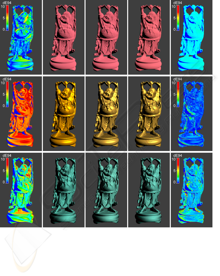
Figure 3: Comparison of factorization with D-BRDF fit under illuminant CIE D65. For each row the middle image is the
reference solution (5nm point sampling), the two images to the left are D-BRDF fit and error, the two to the right show tensor
factorization and error. The error-plots use the ∆E
∗
94
formula of the CIE94 color difference model (McDonald and Smith,
1995). A ∆E
∗
94
under 2 contains an almost unseeable color variance, a ∆E
∗
94
of 5 is clearly noticeable, but the two colors are
still similar, a ∆E
∗
94
above 5 is seldom tolerated. Top row: Oren-Nayar BRDF, σ = 0.52, spectrum is ColorChecker patch 9.
Middle row: Ashikhmin-Shirley BRDF, e
u
= e
v
= 32, spectrum is ColorChecker patch 12. Bottom row: Ashikhmin-Shirley
BRDF, e
u
= 1, e
v
= 8, spectrum is ColorChecker patch 6.
diffuse and glossy part into a single microfacet distri-
bution, which leads to large overall error.
The last row in Fig. 3 shows an anisotropic
Ashikhmin-Shirley BRDF with e
u
= 1, e
v
= 8 (no
diffuse component). The spectrum is ColorChecker
patch 6. For this example we used the HD parameteri-
zation and tabulated the data as a 90×45×90×45×8
five-way tensor. Because the anisotropy adds a mode
for φ
i
to the tensor, more factor packs are needed than
for the isotropic BRDFs. The image was rendered us-
ing 48 factor packs at 18 FPS.
We already mentioned that highly glossy and
GRAPP 2010 - International Conference on Computer Graphics Theory and Applications
170

0.1
0.2
0.3
60
30
0
30
60
90
90
red fabric
0.1
0.2
0.3
0.4
0.5
60
30
0
30
60
90
90
blue metallic paint
0.2
0.4
0.6
0.8
1
60
30
0
30
60
90
90
yellow matte plastic
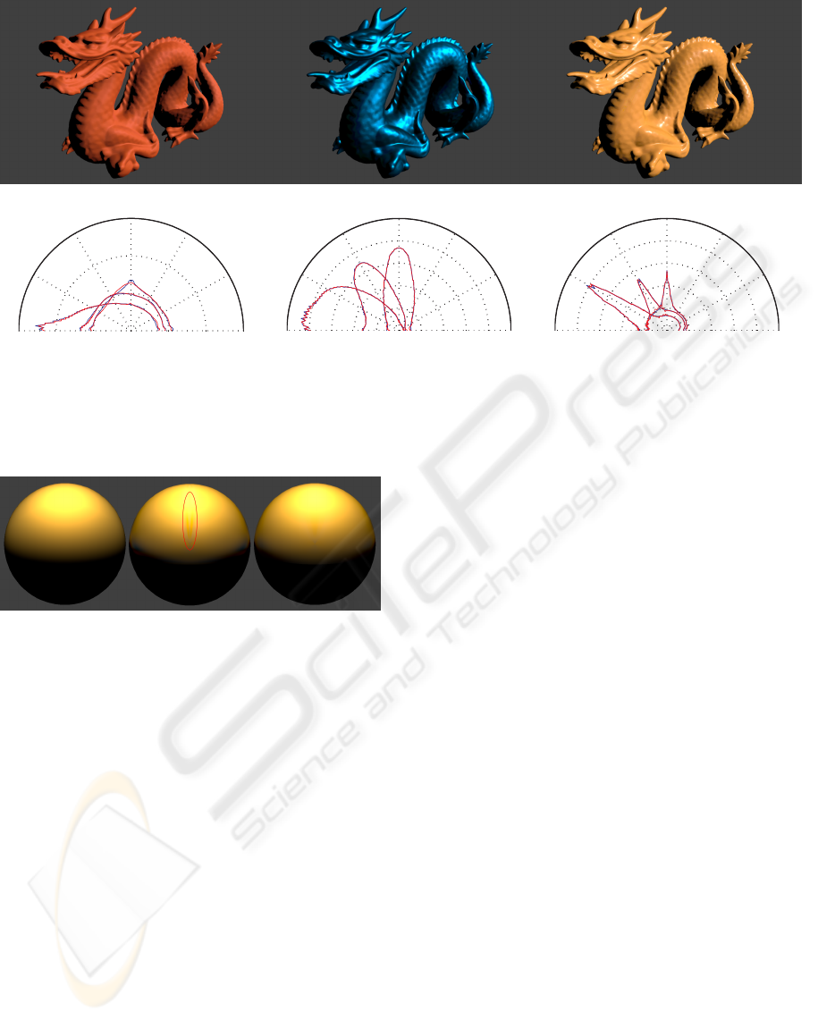
Figure 5: Top: Rendering of measured BRDFs (courtesy of MERL) under CIE D65. From left to right: red fabric (8 factor
packs), blue metallic paint (24 factor packs), yellow matte plastic (22 factor packs). Bottom: Plots of the BRDFs shown in
top row in the plane of incidence for three incident directions (0
◦
, 30
◦
, and 60
◦
incidence from the right) for λ = 550nm.
Measured data is blue, approximation is red. To improve readability we used lines instead of points to plot the data. We also
applied a square root to decrease the extent of the specular lobes in comparison to the diffuse component.
Figure 4: Artifacts can occur for glossy BRDFs if too few
factor packs are used. Left: Reference (Ashikhmin-Shirley
BRDF with e
u
= e
v
= 8, spectrum of ColorChecker patch
12). Middle: In IO parameterization artifacts tend to man-
ifest themselves in the marked area between ω
i
and ω
o
(10
factor packs used). Right: Smoothing the factor packs can
reduce the artifacts without performance impact. In this
case a simple moving average filter (4 tabs wide) was used.
anisotropic BRDFs need many factor packs and that
efficiency is reduced for this class of BRDFs. Another
problem with these BRDFs that we encountered dur-
ing our tests is that the approximation error tends to
manifest itself as artifacts. Usually these artifacts can
be overcome by investing more factor packs, but for
glossy BRDFs convergence is often very slow and us-
ing enough factors to eliminate the artifacts can have
a significant performance impact. If one is not will-
ing to sacrifice performance, a pragmatic approach to
alleviate this issue is to apply a smoothing filter to
the factors (Fig. 4). This will blur the approximation
slightly and make it visually less objectionable, but at
the same time less accurate. Note that apart from Fig-
ure 4 all renderings in this paper did not use a smooth-
ing of the factor packs.
4.2 Measured RGB Data
Because the MERL data base contains only RGB
data, we had to convert these measurements to
spectral BRDFs. We used Smit’s conversion
method (Smits, 1999), which constructs physically
plausible reflectance spectra from RGB values, al-
though when converted back, they usually do not re-
sult in the same RGB triplets. Using Smit’s method
we constructed 90 × 180 × 90 × 61 four-way tensors
in IO parameterization from the MERL BRDFs. So
we have tabulated each BRDF with 1
◦
resolution for
θ
i
, θ
o
, 2
◦
for φ
o
, and 5nm for λ. We then applied
Peercy’s Linear Model as secondary basis and com-
pressed all spectra with 8 basis vectors prior to the
tensor factorization.
Figure 5 shows renderings of three BRDFs with
increasing glossiness and plots of the original data
and the approximation for three incident angles. With
our GPU-based renderer we cannot render tabulated
data sets of this size directly, so we cannot present a
visual comparison here. The number of factor packs
was chosen for each BRDF individually by adding
factor packs until no difference was noticeable in the
result. The plots indicate a very good match.
In general our observation that glossy materials
need more factor packs than mostly diffuse ones was
confirmed. Of the three BRDFs shown in Figure 5,
‘blue metallic paint’ needed the most factor packs
to reach visual convergence, although ‘yellow matte
plastic’ has a narrower specular lobe. We suspect this
MODELING WAVELENGTH-DEPENDENT BRDFS AS FACTORED TENSORS FOR REAL-TIME SPECTRAL
RENDERING
171

is due to the more complex behavior in the spectral
domain inside the main specular lobe of ‘blue metal-
lic paint’.
5 SUMMARY AND OUTLOOK
We presented a method that uses tensor factoriza-
tion to model mostly diffuse and moderately glossy
isotropic spectral BRDFs for real-time rendering on
modern graphics hardware. It can handle high-
resolution tabulated BRDFs, including non-reciprocal
ones, which makes it well-suited for measured data.
One area of application for our research is virtual de-
sign applications that require high color fidelity at in-
teractive frame rates.
With future work, we would like to evaluate our
approach with BRDFs that exhibit more complex in-
teraction between the spectral and spatial domains,
like fluorescent, pearlescent, and ‘flip-flop’ paints.
We are also working on integrating image based light-
ing and precomputed radiance transfer into our spec-
tral renderer.
ACKNOWLEDGEMENTS
The ‘dragon’ and ‘happy buddha’ models used in
this paper are courtesy of the Stanford 3D Scanning
Repository. The first author was partly funded by
BMBF under FKZ 01IM08002E.
REFERENCES
Ashikhmin, M. and Shirley, P. (2000). An anisotropic phong
brdf model. Journal of Graphics Tools, 5(2):25–32.
Claustres, L., Barthe, L., and Paulin, M. (2007). Wavelet
encoding of brdfs for real-time rendering. In GI ’07:
Proceedings of Graphics Interface 2007, pages 169–
176. ACM.
Claustres, L., Boucher, Y., and Paulin, M. (2002). Spec-
tral brdf modeling using wavelets. In Proceedings of
SPIE, Wavelet and Independent Component Analysis
Applications IX, pages 33–43. SPIE.
Duvenhage, B. (2006). Real-time spectral scene lighting on
a fragment pipeline. In SAICSIT ’06, pages 80–89.
South African Institute for Computer Scientists and
IT.
Furukawa, R., Kawasaki, H., Ikeuchi, K., and Sakauchi, M.
(2002). Appearance based object modeling using tex-
ture database. In EGRW ’02, pages 257–266. Euro-
graphics Association.
Harshman, R. A. (1970). Foundations of the PARAFAC
procedure: Models and conditions for an ”explana-
tory” multi-modal factor analysis. UCLA Working Pa-
pers in Phonetics, 16(1):84.
Johnson, G. M. and Fairchild, M. D. (1999). Full-spectral
color calculations in realistic image synthesis. IEEE
Computer Graphics and Applications, 19(4):47–53.
Kautz, J. and McCool, M. D. (1999). Interactive rendering
with arbitrary brdfs using separable approximations.
In SIGGRAPH ’99: Conference abstracts and appli-
cations, page 253. ACM.
Kolda, T. G. and Bader, B. W. (2009). Tensor decomposi-
tions and applications. SIAM Review, 51(3):455–500.
Matusik, W., Pfister, H., Brand, M., and McMillan, L.
(2003). A data-driven reflectance model. ACM Trans-
actions on Graphics, 22(3):759–769.
McDonald, R. and Smith, K. J. (1995). CIE94 - a new
colour-difference formula. Journal of the Society of
Dyers and Colourists, 111(12):376–379.
Munsell Color Science Laboratory (2009). Spec-
tral reflectance of macbeth color checker patches.
http://www.cis.rit.edu/mcsl/.
Oren, M. and Nayar, S. K. (1994). Generalization of lam-
bert’s reflectance model. In SIGGRAPH 94, pages
239–246. ACM Press.
Peercy, M. S. (1993). Linear color representations for full
speed spectral rendering. In SIGGRAPH ’93, pages
191–198. ACM.
Rougeron, G. and Proche, B. (1998). Color fidelity in com-
puter graphics: A survey. Computer Graphics Forum,
17(1):3–15.
Ruiters, R. and Klein, R. (2009). Btf compression via sparse
tensor decomposition. Computer Graphics Forum,
28(4):1181–1188.
Rusinkiewicz, S. M. (1998). A new change of variables for
efficient brdf representation. In EGWR ’98, pages 11–
22. Eurographics Association.
Smits, B. (1999). An rgb-to-spectrum conversion for re-
flectances. Journal of Graphics Tools, 4(4):11–22.
Vasilescu, M. A. O. and Terzopoulos, D. (2004). Tensortex-
tures: multilinear image-based rendering. ACM Trans.
Graph., 23(3):336–342.
Ward, G. and Eydelberg-Vileshin, E. (2002). Picture perfect
RGB rendering using spectral prefiltering and sharp
color primaries. In EGRW ’02, pages 117–124. Euro-
graphics Association.
GRAPP 2010 - International Conference on Computer Graphics Theory and Applications
172