FROM AERIAL IMAGES TO A DESCRIPTION

OF REAL PROPERTIES

A Framework

Philipp Meixner and Franz Leberl

Institute for Computer Graphics and Vision, University of Technology, Inffeldgasse 16, 8010 Graz, Austria

Keywords: Aerial images, 3D-buildings, Image segmentation, Building floors, Window detection, Real property.

Abstract: We automate the characterization of real property and propose a processing framework for this task.

Information is being extracted from aerial photography and various data products derived from that

photography in the form of a true orthophoto, a dense digital surface model and digital terrain model, and a

classification of land cover. To define a real property, one has available a map of cadastral property

boundaries. Our goal is to develop a table for each property with descriptive numbers about the buildings,

their dimensions, number of floors, number of windows, roof shapes, impervious surfaces, garages, sheds,

vegetation, the presence of a basement floor etc.

1 REAL PROPERTIES

We define a “real property” by one or sometimes

multiple parcels as they are recorded in cadastral

maps. It consists of a piece of land, sometimes

defined by a fence, on that land are one or more

buildings, impervious surfaces, garages, trees and

other vegetation. A property may also contain only

the portion of a building, for example in dense urban

cores where buildings are connected.

The description of a real property consists of a

table with coordinates and other numbers. These

define how many buildings exist, the type of

building from a stored list of candidates, building

height and footprint, number of floors, number and

types of windows, presence of a basement floor,

type of attic, roof type and roof details such as an

eave, skylights, chimneys, presence of a garage and

its size, types and extent of impervious surfaces such

a driveway and parking spaces, and statements about

the type and size of elements of vegetation, the

presence of a water body, the existence and type of a

fence etc.

A low cost solution seems feasible if one

considers the wealth of aerial image source data

currently being assembled for other applications, not

insignificantly in connection with innovative

location-aware Internet sites such as Google Maps,

Microsoft Bing-Maps and others.

This paper presents a framework for processing

steps that are necessary for a reasonable semantic

interpretation and evaluation of real property using

high resolution aerial images. Our initial focus is on

characterizing individual properties and their

buildings. This paper illustrates a set of work steps

to arrive at a count of floors and windows.

2 LOCATION-AWARE INTERNET

2.1 Geodata for Location-Awareness

A location-aware Internet (Leberl, 2007) has

evolved since about 2005. Internet-search has been a

driving force in the rapid development of detailed 2-

dimensional maps and also 3-dimensional urban

models. “Internet maps” in this context consist of the

street-maps used for car navigation, augmented by

addresses, furthermore the terrain shape in the form

of the Bald Earth and all this being accompanied by

photographic texture from ortho photos. This is what

is available for large areas of the industrialized

World when calling up the websites

maps.google.com or www.bing.com/maps, and in

some form, this is also available under

www.mapquest.com, maps.yahoo.com or

maps.ask.com, as well as from a number of regional

Internet mapping services.

283

Meixner P. and Leberl F. (2010).

FROM AERIAL IMAGES TO A DESCRIPTION OF REAL PROPERTIES - A Framework.

In Proceedings of the International Conference on Computer Vision Theory and Applications, pages 283-291

DOI: 10.5220/0002817602830291

 SciTePress

Ubiquitous visibility of Geodata started with the

development of car navigation systems for regular

passenger cars. It signaled for the first time a

transition from experts to everyone. The transition

from being a tool for mere trip planning and address

searches to true real-time navigation needed the GPS

to become available, and that was the case since the

mid 1990’s.

“Urban Models” in 3D have been a topic of

academic research since the early 1990’s (Gruber,

1997). As part of Internet mapping, this came into

being in November 2006 with Microsoft’s

announcement of the availability of Virtual Earth in

3D. The vertical man-made buildings are modeled as

triangulated point clouds and get visually

embellished by photographic texture. Since April

2008, vegetation is being classified and identified,

and computer-generated vegetation is being placed

on top of the Bald Earth.

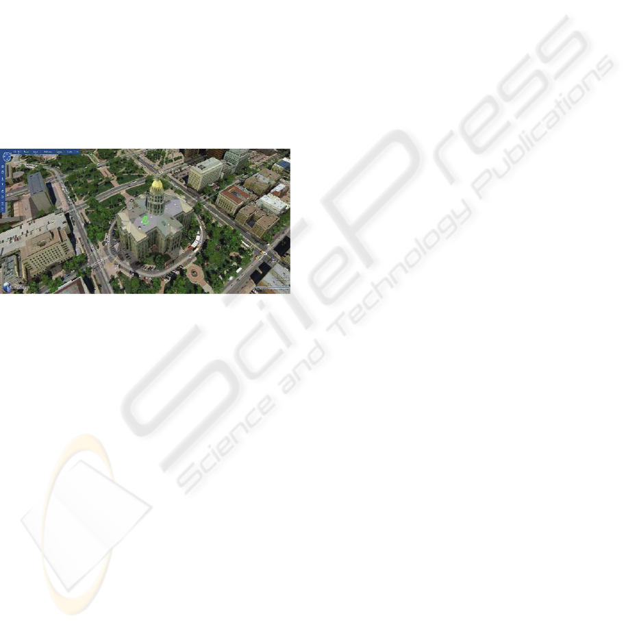
Figure 1: Typical 3D content in support of an Internet

search. Capitol in Denver (Microsoft’s Bing-Maps).

The 3D urban models still are in their infancy

and are provided over large areas only by the

Microsoft-web site Bing/Maps, with an example

presented in Figure 1. While Internet-search may be

the most visible and also initial driving application,

there of course are others. Often mentioned are city

planning, virtual tourism, disaster preparedness,

military or police training and decision making or

car navigation.

2.2 Interpreted Urban Models

The 3D-data representing the so-called location

awareness of the Internet serve to please the user’s

eye – one could speak of “eye candy” -- but cannot

be used as part of the search itself. This is unlike the

2D content with its street map and address codes that

can be searched. An interpreted urban 3D model

would support searches in the geometry data, not

just in the alphanumeric data. One may be interested

in questions involving intelligent geometry data.

Questions might address the number of buildings

higher than 4 floors in a certain district, or properties

with a built-up floor area in excess of 100 m2, with

impervious areas in excess of 30% of the land area,

or with a window surface in excess of a certain

minimum.

Such requirements lead towards the

interpretation of the image contents and represent a

challenge for computer vision (Kluckner, Bischof,

2009).

While currently driven by “search”, applications

like Bing-Maps or Google Earth have a deeper

justification in light of the emerging opportunities

created by the Internet-of-Things and Ambient

Intelligence. These have a need for location

awareness (O’Reilly & Batelle, 2008).

3 A PROCESSING FRAMEWORK

We start out by conflating (merging) geometric data

from two sources: the aerial imagery and the

cadastral information. Figure 2 is an example for a

400 m x 400 m urban test area in the city of Graz

(Austria). Conflation defines each property as a

separate entity for further analysis. Conflation is part

of a pre-processing workflow and results in all

geometric data to be available per property and in a

single geometric reference system.

We now proceed towards the use of the dense 3D

point clouds associated with the aerial photography

and extracted from it by means of a so-called dense

matcher applied to the triangulated aerial

photographs (Klaus, 2007). First is the extraction of

data per building and per element of vegetation. This

finds the areas occupied by a building as well as its

height. For vegetation we need to find the type, its

location, the height and the crown diameter. The

building footprints get refined vis-à-vis the cadastral

prediction using image segmentation and

classification to define roof lines.

From the building one proceeds to the facades:

building footprints become façade baselines. This

footprint is the basis for an extraction of the façade

in 3D by intersecting it with the elevation data. We

compute the corner points of each façade. These can

then be projected into the block of overlapping aerial

photography. We can search in all aerial images for

the best representation of the façade details; we

prepare for a multi-view process.

What follows is a search for rows and columns

of windows in the redundant photographic imagery.

First of all, this serves to establish the number of

floors. Second, we also are interested in the window

locations themselves, as well as in their size. And

VISAPP 2010 - International Conference on Computer Vision Theory and Applications

284

finally, we want to take a look at attics and basement

windows to understand whether there is an attic or

basement.

Figure 3 summarizes the workflow towards a

property characterization and represents the

framework in which the effort is executed.

While an Internet application exists in the USA

that associates with each property a value

(www.zillow.com), this is based on public property

tax records and no information is being extracted

from imagery.

4 SOURCE DATA

4.1 Many Sources for Geo-Data

The diversity of geo-data is summarized in Table 1.

It associates with each type of data source a

geometric resolution or accuracy.

Table 1: The major sources of urban geo-data and their

typical geometric resolution.

The geometry of large urban areas is defined by

aerial photography. While it may be feasible that a

continuous future stream of perennially fresh

GPS/GNSS-tagged collections of crowd-sourced

imagery will do away with any need for aerial

photography, that time has not yet arrived. A

coordinate reference is thus being established by an

automatically triangulated block of aerial

photographs to within a fraction of a pixel across an

entire urban space. Scholz and Gruber (2009)

presented the triangulation results for the aerial

images in the demo set to be within ± 0.5 pixels or ±

5 cm.

4.2 Aerial Images

In the current application, we process aerial images

taken by the large format digital aerial camera

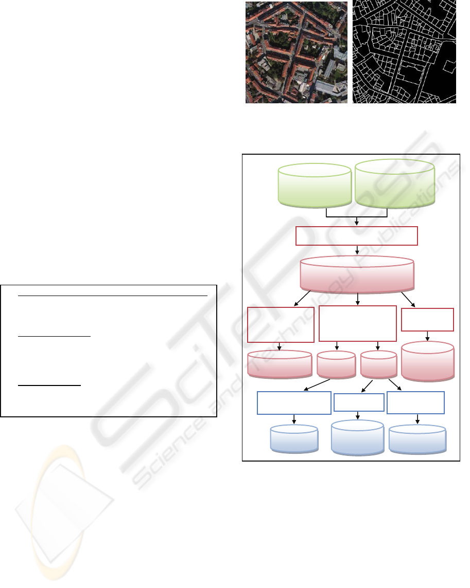
Figure 2: Left is a True Orthophoto of the city of Graz,

400 m * 400 m, at a ground sampling distance of 10 cm.

Right is a cadastral map of Graz [Courtesy BEV-Austria].

Figure 3: Diagram of the proposed work flow to

characterize real properties from aerial images and

associated cadastral data.

UltraCam-X (Gruber et al., 2008). This, like most

digital aerial cameras, produces images in the 4

colors red, green, blue and near infrared (NIR) and

also collects a separate panchromatic channel. The

images often have ~ 13 bits of radiometric range;

this is encoded into 16 bits per color channel. The

entire administrative area of the city of Graz consists

of 155km² and covers the dense urban core and rural

outlying areas. Of this surface area, a total of 3000

aerial photographs have been flown with an along-

track overlap of 80% and an across-track overlap of

Numberandlocation

ofwindows

Floor number

RoofDetailsper

building

Locationofgarages,

baysandtypeofstucco

Windowdetection,

floordetermination

Determinationofroofdetails

Rooftype,Eaves,Skylights,

Chimneys,Typeofattic

Detectionofother

façadedetails

Garages,bays,stucco

Facadesper

building

Location,SizeandTypeof

TreesandHedges

Roofsper

building

Locationandsizeof

impervioussurfaces,

swimmingpools,etc.

Cadastre(GaussKrueger)

StreetNetworks(Display

CoordinateSystem

AerialImages,DTM/DSM

Orthophoto,AT

SegmentedImages

(

WGS84CoordinateS

stem

)



AssemblingDataper property

ChamferMatchin

andCoordinateTransformations

Semanticdescriptionperproperty

Façadedetermination(2Dand3D)

Decomposingofcomplexbuildings

intoseparateobjects

DeterminationofBuildingheights

TreeandVegetation

Detection

Heightsandcrowndiameter

TypeofTree(conifer,

broadleaf)

Determinationof

impervioussurfaces,

waterbodies,etc

ClassifiedImageSegmentsperpropertyandper

building

DTM

DSM

Ortho

hoto

Se

mentedIma

es

OVERHEAD SOURCE URBAN GSD

1. Satellite Imagery 0.5 m

2. Aerial Imagery 0.1 m

3. Aerial Laser Scanning (LIDAR) 0.1 m

STREET SIDE SOURCES

4. Street Side Imagery from Industrial Systems 0.02 m

5. Street Side Lasers 0.02 m

6. Crowd-Sourced Images (FLICKR, Photosynth) 0.02 m

7. Location Traces from Cell Phones and GNSS/GPS 5 m

OTHER DOCUMENTS

8. Cadastral Maps, Parcel Maps 0.1 m

9. Street Maps from Car Navigation 5 m

10. Address codes with geographic coordinates (urban area) 15 m

FROM AERIAL IMAGES TO A DESCRIPTION OF REAL PROPERTIES - A Framework

285

60%, and the Ground Sampling Distance GSD is at

10cm. It should be noted that this large number of

aerial photographs far exceeds, by an order of

magnitude, what one would have flown with a film

camera for manual processing. The overlaps would

have been at 60% and 20%, and the geometric GSD

would have been selected at 20 cm, in order to keep

the cost for film and for manual processing per film

image at affordable levels.

Standard photogrammetric processing is being

applied to such a block of digital photography using

the UltraMap-AT processing system. Full

automation is achieved first because of the high

image overlaps; a second factor is the use of a very

much larger number of tie-points than traditional

approaches have been using.

4.3 DSM and DTM Data

The Digital Surface Model DSM is created by

“dense matching”. The input consists of the

triangulated aerial photographs. In the process, one

develops point clouds from subsets of the

overlapping images and then merges (fuses) the

separately developed point clouds of a given area.

The process is by Klaus (2007). The postings of the

DSM and DTM are at 2 pixel intervals, thus far

denser than traditional photogrammetry rules would

support. The conversion of the surface model DSM

into a Bald Earth Digital Terrain Model DTM is a

post-process of the dense matching and has been

described by Zebedin et al. (2006).

4.4 True Orthophoto

The DSM is the reference surface onto which each

aerial photograph gets projected. The DSM and its

associated photographic texture are then projected

vertically into the XY-plane and result in what is

denoted as a “true” orthophoto. In this data product,

the buildings are only shown by their roofs, not,

however by their facades. Given the overlaps of the

source images, the orthophoto can get constructed

such that all occlusions are being avoided. Image

detail in the orthophoto is therefore taken from

multiple aerial images in a manner that would not be

customary in traditional film-based

orthophotography.

4.5 Image Classification

Any urban area of interest is being covered by

multiple color aerial images. These can be subjected

to an automated classification to develop

information layers about the area. We consider these

to be an input into our characterization procedures.

The classification approach used here has been

described by Zebedin et al. (2006). However,

classification and segmentation methods are topics

of intense research. For example Kluckner, Bischof

(2009) have proposed Random Forests as an

alternative novel method with good results

specifically interpreting urban scenes imaged by the

UltraCam digital aerial camera.

Standard classifications of 4-channel digital

aerial photography typically leads to 7 separate areas

for buildings; grass; trees; sealed surfaces; bare

Earth; water; other objects shown as “unclassified”.

The unclassified areas may show lamp posts, cars,

buses, people etc.

4.6 Cadaster

Since a “property boundary” is a legal concept, it is

not typically visible in the field and from the air

(Fig. 2 right). Also image segmentation algorithms

cannot properly distinguish between buildings when

they are physically attached to one another. It will be

the rare exception that attached buildings can be

separated from aerial imagery, for example if the

roof styles differ, building heights vary or the colors

of the roofing tiles differ. Obviously then, one needs

to introduce the cadastral map.

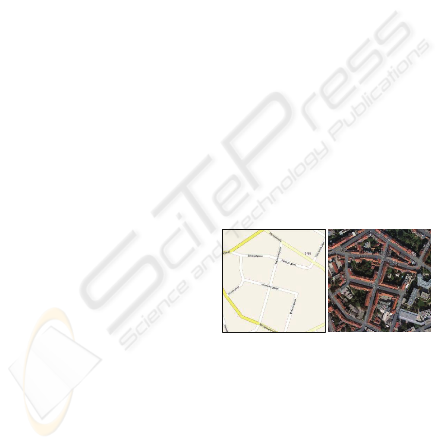
Figure 4: Street layer from car navigation, also from Bing-

Maps (left). Overlay with orthophoto (right), demo Graz.

The cadastral accuracy is being quoted at ± 15cm

which is at the range of the aerial photography’s

pixel size and thus sufficient for the purpose of

characterizing real properties, in accordance with

legislated standards.

4.7 Comments

Car navigation has been the driver for the global

development of street maps. As a result, such data

are available everywhere on the Internet. Figure 4

VISAPP 2010 - International Conference on Computer Vision Theory and Applications

286

illustrates that the street layer does define properties

against the public spaces, and can help in assessing

the traffic issues for a given property.

All source data for the proposed property work

are the result of extensive computation and data

processing, some of it constituting the outcome of

considerable and recent innovations, such as dense

matching and fully automated triangulation.

However, none of that processing is specific to the

property characterization, and therefore is outside

this application.

Much diversity has been and continues being

developed in Geodata sources. There is considerable

discussion about Google’s involvement and its

activities in driving along all roads, even rural ones,

to develop not only a road network but all the

associated addresses. Additionally, there is much

talk about crowd sourced imagery, as typified by

FLICKR, and about information contributed by

users being denoted “neo-geographers”.

5 DATA PER PROPERTY

5.1 Chamfer-Matching

Most cadastral maps, and so also the Austrian

cadastre, basically present a 2D data base and ignore

the 3rd dimension. This causes issues when relating

the cadastral data to the aerial photography and its

inherently 3D data products. In order to co-register

two 2D data sets, an obvious approach is a match

between the 2D-cadastral map with the 2D-

orthophoto. Once this co-registration is achieved, the

cadastral data are also geometrically aligned with all

the other photo-derived data sets.

A 2-step process serves to match the cadastral

map with its own coordinate system with the

orthophoto in its different coordinate reference. In a

first step, the cadastral point coordinates simply get

converted from their Gauss-Krüger M34 values to

the orthophoto’s Universal Transverse Mercator

UTM- system. In an ideal world, this would solve

the registration problem. It does not. There exist

small projection errors that can be seen in a segment

in Figure 5 taken from the demonstration area.

Local shifts in the range of a few pixels, thus some

tens of centimeters, need to be considered.

5.2 Data per Property

The image classification result is in the same

coordinate system as the orthophoto. Therefore the

cadastral map can be used directly to cut a

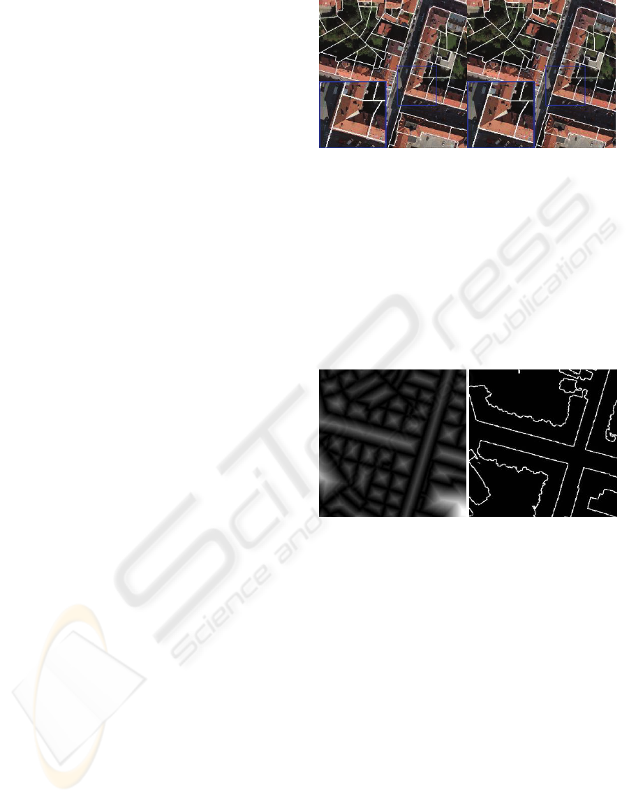
Figure 5: Overlaying the cadastral map over the

orthophoto will leave some small errors that need to be

found and removed. Left after step1, right after step 2.

classification map into data per property. Figure 7

illustrates the result.

A second step is thus needed to achieve a fine

alignment of the Cadastre and the Orthophoto. This

adjustment is accomplished by a so-called Chamfer

Match, here implemented after Borgefors (1988);

Figure 6 illustrates the approach. Figure 5 shows

discrepancies are reduced from their previous ± 7

pixels down to a mere ± 3 pixels.

Figure 6: Cadastral raster distance image (left) and edge

image (right) for a chamfer match.

Zebedin et al. (2006) deliver an accuracy of 90%.

This is consistent with the current effort’s

conclusion. A source for discrepancies between

cadastre and image is seen where the cadastral

boundary line coincides with a building façade. One

observes the existence of façade details such as

balconies, or roof extensions in the form of eaves.

Having the cadastre available offers one the option

of changing the segmentation and classification.

5.3 Dense Point Clouds

In the current test area, the DSM/DTM are an

elevation raster in the coordinate system of the

photogrammetric block and at a posting interval of

20 cm. Cutting the large area dense DSM/DTM data

set along property boundaries is trivial and based on

the cadastral data after Chamfer refinement. Figure 7

contains an illustration of the result.

FROM AERIAL IMAGES TO A DESCRIPTION OF REAL PROPERTIES - A Framework

287

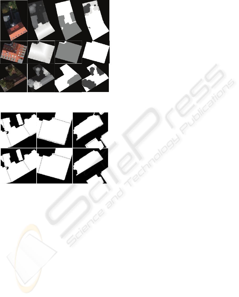
(a) Orthophoto (b) DSM (c) classified buildings (d) classified vegetation

Figure 7: Three separate sample properties and the source

data per property.

Figure 8: Overlay of segmented image and cadastre for

areas in Figure 8. Above is with the discrepancies due to

roof eaves and façade detail, below is a manually cleaned-

up version.

6 PROPERTY DESCRIPTION

Several descriptions have become available as a

byproduct of conflating the 2D cadastral data with

the 2D imagery. We have not only defined the

properties, but in the process we learned their land

area, also the areas used up by the various object

classes such as building, vegetation, water bodies or

impervious surfaces. These measurements of surface

area have previously been determined to be available

at an accuracy of 90%.

However, we have yet to introduce into the work

the 3rd dimension in the form of the dense point

cloud. This will add the most relevant information

These considerations create the need for methods

to automatically improve the alignment of the

cadastral line work and the segmentation boundaries.

Until such algorithms get developed and

implemented, we perform such improvements by

hand. Figure 8 illustrates the discrepancies and their

removal.

The overriding role is associated with the

buildings, and these are in the initial focus of the

effort. All the work being applied is per property.

6.1 Facades Footprint 2D

Vectorizing the Building Contour. The building

objects obtained from the image classification are an

approximation of the intersection of a façade with

the ground. One needs to isolate the contour of each

building object in a given property. Initially, this

contour is in the form of pixels in need of a

vectorization. This is a well developed capability,

one therefore has a choice of approaches. The

Douglas-Peucker algorithm (Douglas, Peucker,

1973) is being used here. The goal is to replace the

contour pixels by straight lines, each line defining a

façade.

Vectorizing the Points along the Vertical

Elements in the DSM. Separately, the 3D point

cloud found for a building object also is a source for

façades. Passing over the X-rows and Y-columns of

the point cloud, one finds the building outline from

the first derivative of the z-values – they represent

the tangent to the point cloud and where this is

vertical, a façade is present.

Reconciling the Segmentation Contour with the

DSM Facade Points. The façade footprints from the

image classification are based on color and texture

and need to be reconciled with the footprint based on

the 3D point cloud. One approach is to define the

mean between the two largely independent

measures.

A Property Boundary Cutting though two

Connected Buildings. In the special case where a

property boundary cuts through a building or a pair

of connected buildings, one does not have a façade.

Such cases need to be recognized. An approach is

the use of the 3

dimension, as shown below. The

output of this step is a series of straight line

segments representing multiple facades.

Decomposing a Building into Separate Building

Objects. The option exists to fit into the pattern of

façade footprints a series of predefined shapes of

(rectangular) building footprints. In the process one

hopes to develop a set of separate non-overlapping

basic building objects. The 3rd dimension is being

VISAPP 2010 - International Conference on Computer Vision Theory and Applications

288

considered via roof shapes. Having more than one

local maximum in the roof height is an indication

that the single building should be segmented into

multiple building objects.

6.2 Façades in the 3

Dimension

Along the footprints of the façade one finds

elevation values in the DSM. These do attach to the

façade a 3rd dimension. Depending on the shape of

the roof, a façade could have a complex shape as

well. However, for use as a descriptor one might be

satisfied with a single elevation value for each

façade. We have now defined a vertical rectangle

for each façade footprint.

A refinement would consist of a consideration of

the change of elevations along the façade footprint.

This could be indicative of a sloping ground, or of a

varying roof line, or a combination of both. The

slope of the ground is known from the DTM. The

variations of the roof line are read off the difference

between the DSM and the DTM.

The issue of connected buildings along a

property line exists. One needs to identify such

façade footprints since they are virtual only. Such

facades can be identified via a look at the dense

point cloud. The elevation values above the Bald

Earth along a façade footprint will be zero at one

side of the footprint. If they are not, then buildings

are connected and this façade is only virtual.

6.3 Building and Roof Heights

A building has multiple façades (see Figure 9), and

each façade represents a value for the height of the

building. However, we have not yet considered the

shape of the roof and therefore may get multiple

building heights, depending on the façade one is

considering. Two elevation numbers are desired to

describe the building at a coarse level: we want to

assign a single building height as well as a single

roof height. The building height is the average of

the façade heights. The roof height is the difference

between the highest point in the building’s point

cloud that the previously computed building height.

6.4 Counting Floors and Windows

Conceptually we are dealing with a three-step

process of analyzing each façade. First, we must

project image content onto each façade rectangle or

other façade shape. Therefore the corner points of a

given façade get projected into each aerial

photograph using the poses of the camera. That will

define in each image a certain number of pixels. The

image area with the highest number of pixels is

likely to produce the best façade image. However, in

the interest of using redundancy, we produce

multiple façade images, one each per aerial

photograph that exceeds a minimum image area to

make sense in the further analysis.

Second, the image segments defined in this

manner will have to be subjected to a floor count.

An edge detector is applied to a given façade image

and the edges are used for the floor count. Therefore

the detected horizontal edge values will be

transformed into a binary format and for each row a

summation of the edge values will be performed. In

a next step all the local maxima are detected and out

of them the floors will be determined (see Figure 9).

Third is the definition of all the windows. This

task has recently received some attention, for

example by Čech and Šára (2007). The window

detection uses the normalized horizontal as well as

vertical gradients. Our approach is taken from Lee

and Nevatia (2004). It extracts windows

automatically via a profile projection method from

each of the single façade images. The Prewitt edges

get projected along the rows and columns of the

façade image and the accumulations of the edges

signify the presence or absence of a window row or

window column. We define straight lines along the

boundary of each accumulation, thereby obtaining

likely candidates for window areas in the 2D plane

of the façade. This method is not very accurate when

there are different shapes of windows in the same

column or line. To refine the window locations a one

dimensional search for the four sides of a window is

performed. Hypothesized lines are generated by

moving the line to its perpendicular direction and

test them. The refined position of the window is

where the hypothesized line has the best score for

the window boundary. Details are available from

Lee and Nevatia (2004).

Figure 10 illustrates the result for the example of

one façade, yet multiple images, and indicates that

the window areas do get defined to within ± 3 pixel

in both the horizontal as well as vertical dimensions,

converting to a value of ± 0.3 m vertically and ± 0.3

m horizontally. In the example shown in Figure 11,

all 33 windows of the façade were found in all 4

aerial images. As one can see in Figure 10 also the 6

basement window openings in every façade could be

detected by evaluating their positions and size in the

image. A door is also detected using its size and

location.

FROM AERIAL IMAGES TO A DESCRIPTION OF REAL PROPERTIES - A Framework

289

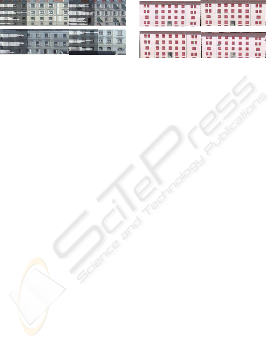
Building 1, Façade 1: (size: 274*100 Pixel) Building 1, Façade 2: (size: 227*100 Pixel)

Building 2, Façade 1: (size: 285*99 Pixel) Building 2, Façade 2: (size: 246*100 Pixel)

Figure 9: One single building has multiple façades.

6.5 Discussion

The approach produces key numbers per building

We also obtain a measure of consistency (a) from

multiple façades for one and the same building and

(b) between the results from multiple overlapping

images (Figure 10). The approach also delivers the

basis for further detail such as shapes and types of

windows, separating façade openings into windows

and doors, defining attic and basement floors. These

key numbers are based on 3D-data about a property

and on the original aerial images showing façade

detail.

Initial work indicates that for some sample

properties like those shown in Figure 7, all floors

and all windows have been found automatically in

each façade, delivering a rather robust result.

Much, however, remains to be done to obtain a

good understanding of the accuracy and reliability of

these key numbers, the problems one will have when

parts of a building are occluded, when the geometric

resolution of the source data varies, when buildings

deviate from a standard shape in the event of add-

ons, have complex footprints and roof shapes, when

cadastral detail contradicts image detail etc.

7 CONCLUSIONS

It is the main purpose of this paper to introduce an

application of vast 3D urban Geodata bases to

automatically characterize real properties. This may

be of value in managing location-based decisions

both in commercial and public interest

environments, and to better administrate municipal

resources. This task is made feasible by the rapid

increase in urban 2D- ad 3D-data which in turn are

being produced in growing quantities for new

applications of the Internet. Global Internet search

providers like Google, Microsoft, Yahoo and Ask all

have developed a mapping infrastructure for

location-aware search systems. They have embarked

on significant efforts to conflate various 2D Geodata

Façade 1: (size: 284*99 Pixel) Façade 2: (size: 285*108 Pixel)

Façade 3: (size 288*125 Pixel) Façade 4: (size: 285*111 Pixel)

Figure 10: One single façade of one single building is

shown four times in overlapping images.

sources, to add business and private address data

bases, parcel data, GNSS and cellular traces and

have started to add the 3rd dimension, both from

aerial as well as street-side images. It is the latter

that is expected to be contributed largely from user-

generated content (UGC). While the initial

battleground for Google and Microsoft is in the

search application, one can already see on the

horizon spatial information as an integral part of the

evolution of the Internet-of-Things (“IoT”) and of

Ambient Intelligence (“AmI”).

To actually succeed in the automated property

description, one will use the original overlapping

aerial images and Geodata derived from the aerial

material. This derived material is in the form of

orthophotos, digital elevation models and pose

information for each aerial photograph. The proposal

presented for an end-to-end property

characterization adds to these data the cadastral

parcel information, and potentially the existing street

maps.

Obviously, one can expect the ease and accuracy

of the data extracted for a property to be a function

of the quality of the source material, in particular of

the elevation data and geometric resolution of the

aerial imagery. While the study of the influence of

source data quality will be a topic for ongoing work,

we already have developed indications that counting

floors and windows poses fairly relaxed demands on

the image quality and pixel size. Initial sample data

on but a few, yet typical properties in an urban core

indicate that all floors and all windows could be

counted correctly.

ACKNOWLEDGEMENTS

Aerial images, DSM, True Orthophotos and

segmented images were provided by Vexcel

Imaging Graz (Microsoft). Help is greatly

appreciated, as provided by B. Gruber, M. Gruber

VISAPP 2010 - International Conference on Computer Vision Theory and Applications

290

(Microsoft), and by M. Donoser, S. Kluckner and G.

Pacher (ICG-TU Graz).

REFERENCES

Borgefors G, 1988: Hierarchical chamfer matching: a

parametric edge matching algorithm, IEEE trans.

Pattern Analysis Machine Intelligence, vol. 10, no. 6,

pp. 849–865.

Čech J., R. Šára (2007) Windowpane detection based on

maximum aposteriori labeling. Technical Report TR-

CMP-2007-10, Center for Machine Perception,

K13133 FEE Czech Technical University, Prague.

Douglas D., T. Peucker (1973), Algorithms for the

reduction of the number of points required to represent

a digitized line or its caricature, The Canadian

Cartographer pp. 112-122.

Gruber M.(1997) Ein System zur umfassenden Erstellung

und Nutzung dreidimensionaler Stadtmodelle,

Dissertation, Graz Univ. of Technology, 1997.

Gruber M., M. Ponticelli, S. Bernögger, F. Leberl (2008)

UltracamX, the Large Format Digital Aerial Camera

System by Vexcel Imaging / Microsoft. Proceedings

of the Intl. Congress on Photogrammetry and Remote

Sensing, Beijing, July 2008

Klaus A. (2007) Object Reconstruction from Image

Sequences. Dissertation, Graz Univ. of Technology,

1997.

Kluckner S., H. Bischof (2009) Semantic Classification by

Covariance Descriptors within a Randomized Forest.

Proceedings of the IEEE International Conference on

Computer Vision, Workshop on 3D Representation for

Recognition (3dRR-09)

Leberl F. (2007) Die automatische Photogrammtrie für

das Microsoft Virtual Earth Internationale

Geodätische Woche Obergurgl. Chesi/Weinold

(Hrsg.), Wichmann-Heidelberg-Publishers, pp. 200-

208

Lee S.C., R. Nevatia (2004) Extraction and Integration of

Window in a 3D Building Model from Ground View

Images. Proc. IEEE Computer Society Conference on

Computer Vision and Pattern Recognition CVP’04

O’Reilly T., J. Batelle (2009) Web Squared: Web 2.0 Five

Years On. O’Reilly Media Inc. Available from

www.web2summit.com.

Scholz S., M. Gruber (2009) Radiometric and Geometric

Quality Aspects of the Large Format Aerial Camera

UltraCam Xp. Proceedings of the ISPRS, Hannover

Workshop 2009 on High-Resolution Earth Imaging for

Geospatial Information, XXXVIII-1-4-7/W5, ISSN

1682-1777

Zebedin L., A. Klaus, B. Gruber-Geymayer, K. Karner

(2006) Towards 3D map generation from digital aerial

images. ISPRS Journal of Photogrammetry and

Remote Sensing, Volume 60, Issue 6, September 2006,

Pages 413-427

FROM AERIAL IMAGES TO A DESCRIPTION OF REAL PROPERTIES - A Framework

291