WIENER-HAMMERSTEIN PARAMETER ESTIMATION USING

DIFFERENTIAL EVOLUTION

Application to Limb Reﬂex Dynamics

Oliver P. Dewhirst, David M. Simpson, Natalia Angarita, Robert Allen

Institute of Sound and Vibration Research, University of Southampton, Southampton, U.K.

Philip L. Newland

School of Biological Sciences, University of Southampton, Southampton, U.K.

Keywords:

Wiener-Hammerstein, Differential evolution, Locust, Limb reﬂex dynamics, Neuromuscular modelling.

Abstract:

The nonlinear Wiener-Hammerstein model, which consists of a static (no memory) non-linearity sandwiched

between two dynamic (with memory) linear elements, provides a parsimonious and accurate model for

representing a number of biological systems. In this study we compare the performance of two Wiener-

Hammerstein parameter estimation methods; a commonly used nonlinear local optimisation method and the

global optimisation method Differential Evolution. The accuracy and convergence properties of the two meth-

ods is tested using experimental data collected from the locusts hind limb reﬂex control system and using

computer simulations.

1 INTRODUCTION

A greater understanding of neuromuscular control of

limb movement is vital for optimising the treatment

of patients with neuromuscular dysfunction. System

identiﬁcation methods provide a valuable tool for in-

vestigating the complex mechanical and neural com-

ponents of such systems (Bai et al., 2009; Dempsey

and Westwick, 2004). Our work uses the locust as

a model system because it provides the opportunity

to develop new system identiﬁcation techniques and

gain physiological insight into a related but simpler

and more accessible system.

Nonlinear Wiener or Volterra seriesmodels, a gen-

eralisation of the convolution integral for a linear sys-

tem, have often been used to model the nonlinear

responses generated by reﬂex limb control systems

(Newland and Kondoh, 1997) and other biological

systems (Song et al., 2009). These series are often

truncated to second order because it is difﬁcult to vi-

sualise, interpret and calculate, in terms of compu-

tational cost and length of data required, the higher

order kernels.

Cascade models, a restricted subset of the Volterra

series, have been shown to provide a parsimonious

and easier to interpret alternative for representing

such systems (Dewhirst et al., 2009; Dempsey and

Westwick, 2004). Cascade models consist of linear

dynamic (with memory) elements and static (no mem-

ory) nonlinear elements. Common conﬁgurations in-

clude the Wiener (linear - nonlinear), Hammerstein

(nonlinear - linear) and the Wiener-Hammerstein (lin-

ear - nonlinear - linear) model shown in Figure 1.

Methods to estimate the parameters of the Wiener-

Hammerstein model are currently receiving much at-

tention for control applications (Schoukens et al.,

2009) but not for application to biological systems.

A key feature of the locust’s hind leg control sys-

tem is a reﬂex control loop. This system uses a me-

chanical loop structure attached to the tibia by an

apodeme to move a stretch sensor called the Femoro-

tibial Chordotonal Organ (FeCO). Sensory neurons in

the FeCO convert mechanical stimuli into electrical

signals which are transmitted to motor neurons which

activate muscle contraction (Newland and Kondoh,

1997). Previous work (Dewhirst et al., 2009) found

that the Wiener-Hammerstein model was the opti-

mum structure for representing the dynamic reﬂex re-

sponse of the Fast Extensor Tibia (FETi) motor neu-

ron in the locusts hind leg control system, the system

studied in the current work.

As the cascade models are nonlinear in their pa-

271

P. Dewhirst O., M. Simpson D., Angarita N., Allen R. and L. Newland P. (2010).

WIENER-HAMMERSTEIN PARAMETER ESTIMATION USING DIFFERENTIAL EVOLUTION - Application to Limb Reﬂex Dynamics.

In Proceedings of the Third International Conference on Bio-inspired Systems and Signal Processing, pages 271-276

DOI: 10.5220/0002741902710276

 SciTePress

Figure 1: The Wiener-Hammerstein model.

rameters and have a differentiable cost function their

parameters can be estimated using a nonlinear local

optimisation method. One of the most widely used

local optimisation methods for estimating the parame-

ters of the Wiener-Hammerstein models for biological

applications was developed by Korenberg and Hunter

(Korenberg and Hunter, 1986) (the KH method). As

the cost function of the model is multi-modal, such

methods require careful parameter initialisation to en-

sure that they do not convergeto a local rather than the

global minimum (Schoukens et al., 2008; Dempsey

and Westwick, 2004).

An alternative approach is to use a nonlinear

global optimisation method such as simulated anneal-

ing which has been developed to avoid the problem

of local minima. As these methods can suffer from

slow convergence and poor local search characteris-

tics their application has often been restricted to ﬁnd-

ing initial parameter estimates for the local methods

(Juusola et al., 2003). One type of evolutionary algo-

rithm, Differential Evolution (DE), however, has been

shown to give fast robust convergence and good lo-

cal search performance. It also requires few control

parameters and is easy to use and implement (Storn

and Price, 1997). DE has been applied to estimate the

parameters of Hammerstein and Wiener models (Al-

Duwaish, 2000) but we do not believe to the Wiener-

Hammerstein model.

In this study we compare the performance of the

DE and KH methods for estimating the parameters

of the Wiener-Hammerstein model from experimental

data obtained from the locusts leg control system and

computer simulations.

2 METHODS

The linear elements of the Wiener-Hammerstein

model (Figure 1) have a Finite Impulse Response

(FIR) structure. A polynomial function was chosen to

represent the static nonlinear element. The noise free

output of the Wiener-Hammerstein model is given by

y(t) =

∑

σ=1

g(σ)

∑

q=0

(q)

∑

τ=1

h(τ)u(t − σ − τ)

(1)

Where T is the length of the FIR ﬁlter and Q is the

polynomial order.

2.1 Differential Evolution

The parameters of the Wiener-Hammerstein model

are coded in a vector containing D elements

x =



h(1), . . . , h(T), c

, . . . , c

, g(1), . . . , g(T)



(2)

Differential Evolution (DE) works with a population,

P, of NP D-dimensional parameter vectors (Storn and

Price, 1997)

(G)







(G)

1,1

(G)

1,2

··· x

(G)

1,D

(G)

2,1

(G)

2,2

··· x

(G)

2,D

(G)

NP,1

(G)

NP,2

··· x

(G)

NP,D







(3)

where x

(G)

1,1

(G)

1,2

···x

(G)

1,D

are elements of x. Each param-

eter vector

(G)



(G)

i,1

, x

(G)

i,2

, . . . ,x

(G)

i,D



i = 1, 2, . . . , NP (4)

represents a possible solution to the optimisation

problem. The population is initialised randomly and

evolves in generations (iterations), G. With each gen-

eration a mutant vector, v

, is formed from each of the

NP parent vectors, x

, following

(G+1)

= x

(G)

+ F



(G)

− x

(G)



(5)

with the multiplication factor F set by the user (F >

0) and random, mutually different indexes r

, r

∈

{1, 2, . . . ,NP} which are also different from i. The

trial vector

(G+1)



(G+1)

i,1

, u

(G+1)

i,2

, . . . , u

(G+1)

i,D



(6)

is generated using the crossover operator

(G+1)

i, j

(

(G+1)

i, j

if (rnd( j) ≤ CR)

(G)

i, j

if (rnd( j) > CR)

(7)

where j = 1, 2, . . . , D and rnd( j) is the j

output from

a random number generator with a uniform distribu-

tion. The cross over constant CR ∈ [0, 1] is set by

the user; rn(k) ∈ {1, 2, . . . , D} is a randomly chosen

index used to ensure that at least one of the parame-

ters from v

i, j

is transferred to u

i, j

. The widely used

Minimum Mean Square Error (MMSE) cost function

is used to compare the performance of the trial and

parent vectors.

J =

N−1

∑

t=0

(z(t) − ˆy(t))

(8)

where N is the signal length in samples. A greedy

selection procedure (does not reconsider past genera-

tions) is used to determine if the parent vector should

BIOSIGNALS 2010 - International Conference on Bio-inspired Systems and Signal Processing

272

be retained for the next generation, or replaced by

the trial vector. These steps are repeated either for a

speciﬁc number of generations or until a certain cost

function value is reached. The DE method was set

up with F = 0.5, CR = 0.9, NP = 10 × D (Storn and

Price, 1997) and was run for 900 iterations.

2.2 The Korenberg Hunter Method

Korenberg and Hunter (Korenberg and Hunter, 1986)

use an iterative two step approach to estimate the pa-

rameters of the Wiener-Hammerstein model. Their

method is summarised in Algorithms 1 and 2.

Algorithm 1. KH parameter estimation.

Require: Initial estimate of

h(τ) = (

, 0, 0, . . . ,0)

1: Filter u(t) by

h(τ) to obtain ˆx(t)

2: Fit the Hammerstein system between ˆx(t) and z(t)

using Algorithm 2

3: If ﬁrst iteration or signiﬁcant improvement in

model accuracy continue, else exit with current

parameters

4: Obtain a new estimate of

h(τ) using the

Levenberg-Marquardt (LM) (Marquardt, 1963)

gradient based method to minimise J (Equation

8) given the current estimate of the Hammerstein

system. Return to step 2

Algorithm 2. Hammerstein parameter estimation.

1: Fit a linear system between z(t) and ˆx(t) to obtain

an initial estimate of the inverse of ˆg(τ), ˆg(τ)

−1

2: Filter z(t) by ˆg(τ)

−1

to obtain ˆw(t)

3: Fit a polynomial ˆm(·) between ˆx(t) and ˆw(t)

4: Obtain a new estimate of ˆw(t) given ˆm( ˆx(t))

5: Re-estimate ˆg(τ) given ˆw(t) and z(t)

6: Calculate the %MSE (Equation 9) difference be-

tween model output ˆy(t) and measured outputz(t)

7: If the %MSE reduction is small compared to last

iteration, exit with current parameters

8: Else, compute a new estimate of ˆg(τ)

−1

using the

current ˆw(t) and z(t). Return to step 2

2.3 Experimental Data

The performance of the two parameter estimation

methods was measured using experimental data col-

lected from the locust (Schistocerca gregaria). A

brief summary of the experimental methods used by

Newland and Kondoh (Newland and Kondoh, 1997)

follows. The locusts were mounted in modelling

clay; the apodeme of the FeCO was exposed by dis-

section and was attached by forceps to an electro-

mechanical shaker (LDS, type 101). The FeCO was

stimulated by applying a 27Hz low pass ﬁltered Gaus-

sian White Noise (GWN) signal to the shaker to move

the apodeme (Figure 2 A). The synaptic inputs to

0 10 20 30 40

120

Time (s)

Joint angle (degs.)

0 10 20 30 40

−0.4

−0.2

0.2

Time (s)

Amplitude (mV)

s1 s2 s3

0 10 20 30 40 50

−60

−40

−20

Frequency (Hz)

Power (dB)

Input

Output

Noise

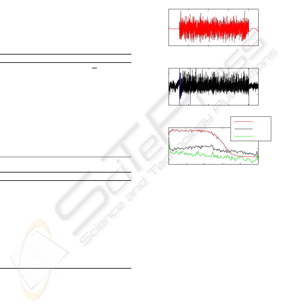
Figure 2: The band limited (0-27Hz) GWN input signal

applied to move the apodeme of the FeCO (A). A typical

output signal recorded from FETi (B). Noise, the transient

adapting response of FETi and its steady state adapted re-

sponse are marked as s1, s2 and s3 respectively. The spec-

trum of the input signal, adapted FETi response (s3) and

noise signal (s1) are plotted in C.

the FETi motor neuron, caused by stimulation of the

apodeme of the FeCO, were measured by inserting a

glass microelectrode into its soma. A typical record-

ing from the soma of the FETi motor neuron is shown

in Figure 2 B. The high level of measurement and

background neural noise, initial transient response

and steady state adapted response of FETi can be

seen in Figure 2 B sections s1, s2 and s3 respectively.

Models were ﬁtted between the ﬁrst 600 samples (6s

with fs=100Hz) of the steady state adapted response

of FETi (Figure 2 B s3) and the corresponding sam-

ples of input signal. The performance of the parame-

ter estimation methods was determined by calculating

the %MSE difference between the predicted output of

the model and the measured output of the neuron us-

WIENER-HAMMERSTEIN PARAMETER ESTIMATION USING DIFFERENTIAL EVOLUTION - Application to

Limb Reflex Dynamics

273

ing 200 samples of validation data.

MSE = 100×

∑

t=1

(y(t)− ˆy(t))

∑

t=1

y(t)

(9)

Before the performance of the two parameter estima-

tion methods was compared, the number of model

parameters was optimised. As six sets of data were

available, six models were estimated using the KH

method. The %MSE performance of each of these

models with a varying number of parameters was cal-

culated, using validation data. The optimum num-

ber of parameters was determined by calculating the

mean of the minimum %MSE value. As the gain of

the locust system can be arbitrarily assigned to the

linear and nonlinear elements of the model these ele-

ments have been normalised to allow comparison.

2.4 Simulations

Computer simulations were used to investigate the

robustness of the two parameter estimation methods

to experimental conditions. The simulated system

was based on one of the Wiener Hammerstein mod-

els identiﬁed from experimental data using the KH

method. Measurement noise coupled with the limited

bandwidth of the input signal (Figure 2 C) introduces

random estimation errors into the linear elements of

the model. As the estimation error occurs where there

is little input power (> 27Hz) and system dynamics it

was removed using a low pass ﬁlter (zero phase, 3

order Butterworth, f

= 27Hz).

“Ideal” and “low pass with measurement noise”

data sets were generated using the simulated system.

To create the “ideal” data set, a GWN signal was gen-

erated and applied to the simulated system. The in-

put signal in the “low pass with measurement noise”

data set represents the input signal used in the locust

experiments. It was created by ﬁltering the GWN in-

put signal with a low pass ﬁlter (zero phase, 5

order

Butterworth, f

= 27Hz). The effect of measurement

noise on the parameter estimation methods was inves-

tigated using a Monte Carlo simulation (100 trials).

In each trial measurement noise with a Gaussian dis-

tribution was added to the output from the simulated

system generated using the same low pass input sig-

nal. The noise was added to give a Signal to Noise

Ratio of 5dB, a level similar to that found in the lo-

cust recordings.

3 RESULTS AND DISCUSSION

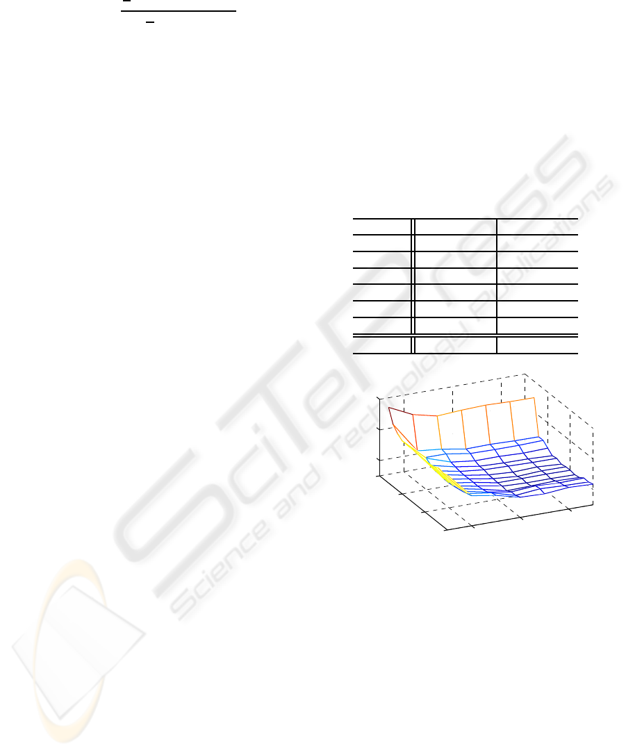
The variation in mean %MSE performance of the

Wiener-Hammerstein model (parameters estimated

using the KH method) with the number of parameters

it contains is plotted in Figure 3. This result shows

that optimum performance is obtained with 9 parame-

ters in each linear element and a 5

order polynomial,

though the minimum is in an almost ﬂat area of the pa-

rameter space. The mean %MSE performance of the

models, containing the optimum number of parame-

ters, with their parametersestimated using the KH and

DE methods is very similar (30.0% and 29.0% respec-

tively, Table 1). Both methods also produce similar

mean parameter estimates (Figure 4).

Table 1: %MSE performance of the Wiener-Hammerstein

models, with their parameters estimated using the KH and

DE methods, on validation data. Models contain the opti-

mum number of parameters.

Animal KH method DE method

1 31.0 29.2

2 29.4 32.4

3 17.6 19.6

4 36.0 33.3

5 32.1 28.0

6 34.1 31.3

Mean 30.0 29.0

↓

Polynomial order (Q)

Total no. of linear

parameters (2T)

%MSE

Figure 3: Mean (n=6) %MSE performance variation for val-

idation data with the total number of linear parameters in the

model and polynomial order. The minimum mean MSE is

30.0% and occurs with a total of 18 linear parameters and a

order polynomial (marked with an arrow).

The non white spectrum of the input signal (Fig-

ure 2 C) coupled with the high levels of measure-

ment noise (Figure 2 B s1) results in the parameter

estimates containing high frequency estimation error

(Figure 4). The rather high %MSE performance of

the models, suggests that they provide a poor ﬁt to

the system. The recordings prior to the start of stim-

ulation, when the input is constant, show consider-

able measurement noise (Figure 2 B s1). Analysis

has shown that the spectrum of the residual signal (the

difference between the model and the measured out-

BIOSIGNALS 2010 - International Conference on Bio-inspired Systems and Signal Processing

274

0 20 40 60 80

−1

−0.5

0.5

Lag (ms)

Amplitude

−1 0 1

−1

−0.5

0.5

Input

Output

0 20 40 60 80

−1

−0.5

0.5

Lag (ms)

Amplitude

Model estimates (6 animals)

Mean of model estimates

0 20 40 60 80

−1

−0.5

0.5

Lag (ms)

Amplitude

−1 0 1

−1

−0.5

0.5

Input

Output

0 20 40 60 80

−1

−0.5

0.5

Lag (ms)

Amplitude

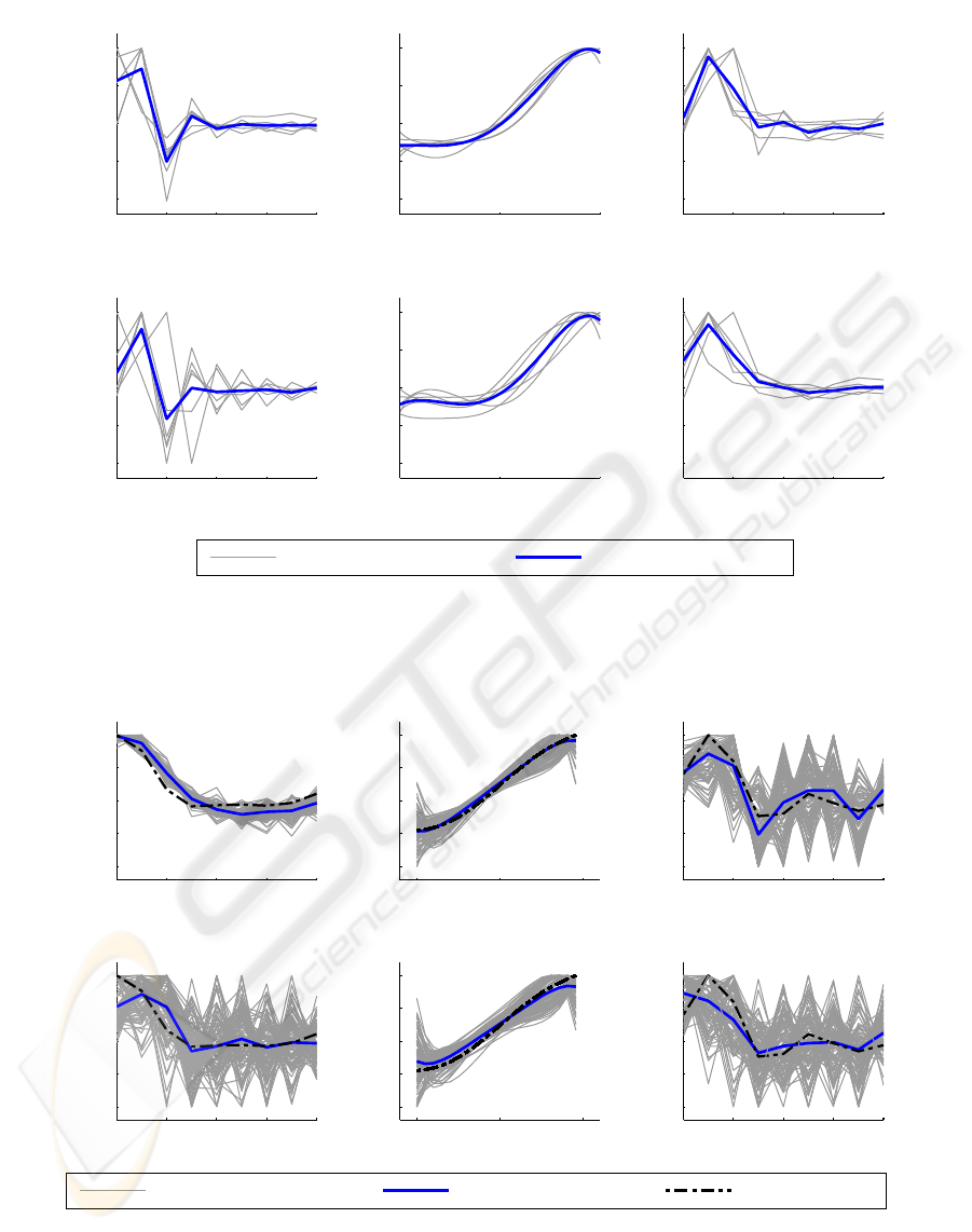
Figure 4: The parameters of the Wiener-Hammerstein models of the FETi system estimated using the KH method (A-C) and

the DE method (D-F). The ﬁrst linear element h(τ) is plotted in A and D, the second linear element g(τ) in C and F. The

polynomial function is plotted in B and E. Note that the parameters have been normalised to allow comparison.

0 20 40 60 80

−1

−0.5

0.5

Lag (ms)

Amplitude

−1 0 1

−1

−0.5

0.5

Input

Output

0 20 40 60 80

−1

−0.5

0.5

Lag (ms)

Amplitude

Model estimates (100 trials)

Mean of model estimates

Simulated system

0 20 40 60 80

−1

−0.5

0.5

Lag (ms)

Amplitude

−1 0 1

−1

−0.5

0.5

Input

Output

0 20 40 60 80

−1

−0.5

0.5

Lag (ms)

Amplitude

Figure 5: Results of Monte Carlo simulations comparing the performance of the KH (A to C) and the DE (D to F) pa-

rameter estimation methods using the “low pass with measurement noise” data set. In each trial measurement noise with

a Gaussian distribution was added to the output of the simulated system generated using the same low pass input sig-

nal.

WIENER-HAMMERSTEIN PARAMETER ESTIMATION USING DIFFERENTIAL EVOLUTION - Application to

Limb Reflex Dynamics

275

put signal) is very similar to the spectrum of the noise

signal. This suggests that model ﬁt is good, as one

cannot expect the model to be able to predict the ran-

dom measurement noise.

Computer simulations using the “ideal” data set

showed that both parameter estimation methods could

accurately identify the simulated system. The nor-

malised parameter bias error for both methods was

less than 0.1%. The results of the Monte Carlo sim-

ulation using the “low pass with measurement noise”

data set are shown in Figure 5. Under these simu-

lated experimental conditions, neither method could

retrieve the parameters of the simulated system. It is

interesting to note that the DE estimates of the pa-

rameters of h(τ) (Figures 4 and 5 D) contain more

high frequencyestimation error than the KH estimates

(Figures 4 and 5 A) for both experimental and simu-

lated data. This is probably because the LM method

(Westwick and Kearney, 2003) used to estimate h(τ)

in the KH algorithm (Algorithm 1 step 4) approxi-

mates the Hessian

H as

H =

J+ µ

(10)

and the µ

term improves the condition of

4 CONCLUSIONS

The accuracy of two Wiener-Hammerstein parame-

ter estimation methods has been compared using ex-

perimental data and computer simulations. Our work

has shown that DE gives fast robust convergence and

good local search performance, providing similar ac-

curacy as the local optimisation method developed by

Korenberg and Hunter (Korenberg and Hunter, 1986).

The DE method offers the advantageof simplicity and

ﬂexibility, for example making it easy to use different

cost functions. Also, as it is a global method, it should

be less sensitive to parameter initialisation, but addi-

tional work is require to verify this feature. Further

investigation into the convergence properties of both

methods and ways to reduce parameter bias and vari-

ance under experimental conditions is required.

ACKNOWLEDGEMENTS

The authors would like to thank the Gerald Kerkut

Trust, the LSI Forum, the ISVR Rayleigh Scholarship

and the BBSRC for their support.

REFERENCES

Al-Duwaish, H. (2000). A genetic approach to the identi-

ﬁcation of linear dynamical systems with static non-

linearities. International Journal of Systems Science,

31(3):307–313.

Bai, E., Cai, Z., Dudley-Javorosk, S., and Shields,

R. K. (2009). Identiﬁcation of a modiﬁed wiener-

hammerstein system and its application in electrically

stimulated paralyzed skeletal muscle modeling. Auto-

matica, 45(3):736 – 743.

Dempsey, E. and Westwick, D. (2004). Identiﬁcation

of hammerstein models with cubic spline nonlinear-

ities. IEEE Transactions on Biomedical Engineering,

51(2):237–245.

Dewhirst, O., Simpson, D., Allen, R., and Newland, P.

(2009). Neuromuscular reﬂex control of limb move-

ment - validating models of the locust’s hind leg con-

trol system using physiological input signals. In IEEE

EMBS 09, 4th International Conference on Neural En-

gineering. IEEE EMBS.

Juusola, M., Niven, J., and French, A. (2003). Shaker

k+ channels contribute early nonlinear ampliﬁcation

to the light response in drosophila photoreceptors. J

Neurophysiol, 90(3):2014–2021.

Korenberg, M. and Hunter, I. (1986). The identiﬁcation of

nonlinear biological systems: lnl cascade models. Bi-

ological Cybernetics, 50(2):125–134.

Marquardt, D. W. (1963). An algorithm for least-squares

estimation of nonlinear parameters. SIAM Journal on

Applied Mathematics, 11(2):431–441.

Newland, P. and Kondoh, Y. (1997). Dynamics of neurons

controlling movements of a locust hind leg iii: Exten-

sor tibiae motor neurons. The Journal of Neurophysi-

ology, 77(5):3297–3310.

Schoukens, J., Pintelon, R., and Enqvist, M. (2008). Study

of the lti relations between the outputs of two coupled

wiener systems and its application to the generation

of initial estimates for wiener-hammerstein systems.

Automatica, 44(7):1654 – 1665.

Schoukens, J., Suykens, J., and Ljung, L. (2009). Wiener

hammerstein benchmark. In Proc. 15 IFAC Sympo-

sium on System Identiﬁcation, St Malo, France.

Song, D., Marmarelis, V., and Berger, T. (2009). Paramet-

ric and non-parametric modeling of short-term synap-

tic plasticity. part i: Computational study. J Comput

Neurosci, 26(1):1 – 19.

Storn, R. and Price, K. (1997). Differential evolution a sim-

ple and efﬁcient heuristic for global optimization over

continuous spaces. Journal of Global Optimization,

11:341–359.

Westwick, D. and Kearney, R. (2003). Identiﬁcation of Non-

linear Physiological Systems. Wiley-IEEE Computer

Society Pr, Piscataway, New Jersey, 1st edition.

BIOSIGNALS 2010 - International Conference on Bio-inspired Systems and Signal Processing

276