PROGNOSIS OF BREAST CANCER BASED ON A FUZZY
CLASSIFICATION METHOD
L. Hedjazi
1,2
, T. Kempowsky-Hamon
1,2
, M.-V. Le Lann
1,2
and J. Aguilar-Martin
1,3
1
CNRS, LAAS, 7, avenue du Colonel Roche, F-31077 Toulouse, France
2
Université de Toulouse, UPS, INSA, INP, ISAE, LAAS, F-31077 Toulouse, France
3
Universitat Politècnica de Catalunya, grup SAC;Rambla de Sant Nebridi, 10, E-08222 Terrassa (Catalunya), Spain
Keywords: Classification, Breast cancer prognosis, Numerical and symbolic data, Fuzzy logic.
Abstract: Learning and classification techniques have shown their usefulness in the analysis of ana-cyto-pathological
cancerous tissue data to develop a tool for the diagnosis or prognosis of cancer. The use of these methods to
process datasets containing different types of data has become recently one of the challenges of many
researchers. This paper presents the fuzzy classification method LAMDA with recent developments that
allow handling this problem efficiently by processing simultaneously the quantitative, qualitative and
interval data without any preamble change of the data nature as it must be generally done to use other
classification methods. This method is applied to perform breast cancer prognosis on two real-world
datasets and was compared with results previously published to prove the efficiency of the proposed
method.
1 INTRODUCTION
In the cancer treatment domain, there are two
distinct purposes: diagnosis of cancer and the
prognosis of survival or relapse/recurrence in the
case of a previously diagnosed cancer. This work
focuses on developing a methodology for the
prognosis to better assess the potential risk of
relapse based on the analysis of ana-cyto-
pathological data. Among many works performed in
the cancer diagnosis field, classical classification
methods often give satisfactory results (Ryu et
al.,2007). However, in the prognosis field, they have
shown a real difficulty in obtaining accurate
predictions in terms of the relapse risk (Holter,
1993). This is due firstly to the fact that the potential
prognostic factors remain still partially known
(Deepa et al., 2005) and, secondly, the data
contained in prognosis datasets are heterogeneous:
they can be quantitative or qualitative and even take
the form of intervals. In this work, the fuzzy
classification method LAMDA based on learning
(Learning Algorithm for Multivariable Data
Analysis) (Aguilar-Martin & López de Mantaras,
1982) was used. LAMDA can handle datasets that
contain simultaneously features of different type:
quantitative, qualitative (Isaza et al., 2004). In the
present paper, this method is also extended in order
to handle another type of data: interval.
The paper is organized as follows: in section 2, a
brief presentation of the general classification
procedure based on the LAMDA method is given
with the treatment of different types of data
(quantitative, qualitative, intervals). In section 3, an
application on two Breast Cancer Prognosis datasets
illustrates the effectiveness of the proposed
methodology. Finally the paper is concluded and
perspectives on future works are given in section 4.
2 CLASSIFICATION
PROCEDURE BY LEARNING
For any classification and analysis method based on
learning, there are two principal phases (Figure 1):
training and recognition (or test). In the training
phase the objective is to find the set of classes (with
their features or their parameters: number, shapes,...)
which represents at best a set of known data. In the
recognition phase new cases (other than those used
for learning) are examined and matched to the
classes obtained during the training phase.
123
Hedjazi L., Kempowsky-Hamon T., Le Lann M. and Aguilar-Martin J. (2010).
PROGNOSIS OF BREAST CANCER BASED ON A FUZZY CLASSIFICATION METHOD.
In Proceedings of the First International Conference on Bioinformatics, pages 123-130
DOI: 10.5220/0002716601230130
Copyright
c
 SciTePress

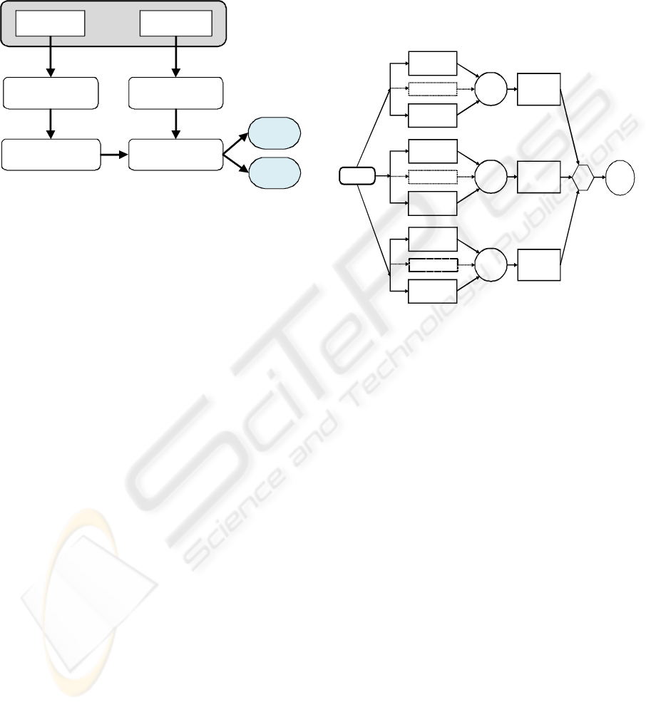
During the training phase, the first step is to
select the features that best discriminate the different
classes (Figure 1). This selection may relate to the
raw data as the results from filtering, principal
components analysis (PCA),.... The next step is to
determine the parameters of each class.
Learning
Data
Validation
Data
Feature selection
Classification
Recognition
(prognosis)
No
Relapse
Relapse
Selected Features
Figure 1: Data processing by classification.
2.1 LAMDA Classification Method
LAMDA is a fuzzy methodology of conceptual
clustering and classification. It is based on finding
the global membership degree of an individual to an
existing class, considering all the contributions of
each of its features. This contribution is called the
marginal adequacy degree (MAD). The MADs are
combined using "fuzzy mixed connectives" as
aggregation operators in order to obtain the global
adequacy degree (GAD) of an element to a class.
LAMDA can simultaneously handle qualitative and
quantitative data (Isaza et al., 2004) and has been
recently extended to interval data.
LAMDA offers the possibility to make a
supervised learning (with classes assigned a priori)
and/or unsupervised (self-learning). Learning is
done in an incremental and sequential way, thus
reducing the learning phase to one or very few
iterations. The assignment of an individual to a class
follows always the same procedure; the present
individual initializes a class or contributes to the
modification of an existing class. Figure 2 illustrates
the procedure for assigning an individual to a class.
LAMDA states upon the assumption that the
features of the elements to be classified are
independent of each other, i.e. there is no correlation
between the variables (features).
2.2 MAD: Marginal Adequacy Degree
The marginal adequacy degree (MAD) is expressed
as a function of marginal relevance to the C
k
class:
μ
k
i
(x
i
) = MAD(x
i
/ i
th
parameter of class C
k
)
This function depends on the i
th
feature x
i
of the
individual X and on parameter
θ
ki
of class C
k
:
μ
k
i
(x
i
) = f
i
(x
i
, θ
ki
)
The parameter
θ
ki
is calculated iteratively from the
i
th
feature of all individuals belonging to class C
k
.
The procedure to calculate the MAD when the
feature is qualitative, quantitative or interval is
detailed in the following subsections.
marginal
membership
feature 1
Fuzzy
connective
Global
Membership
Class 1
MAX
Element X
Assigned
Class
marginal
membership
feature M
marginal
membership
feature 1
Fuzzy
connective
Global
Membership
Class k
marginal
membership
feature M
marginal
membership
feature 1
Fuzzy
connective
Global
Membership
Class K
marginal
membership
feature M
Figure 2: LAMDA structure for 3 classes.
2.2.1 Qualitative Type Features
In the qualitative case, the possible values of the i
th
feature form a set of modalities:
D
i
= {Q
i1
,…Q
ij
,…Q
iMi
}
Let
Φ
ij
be the probability of Q
ij
in the class C
k
,
estimated by its relative frequency, then the
membership function of x
i
is multinomial:
(
)
ΦΦ
∗∗=
iMii
q
iMi
q
i
i
i
k
x
L
1
1
μ
where:
(1)
⎪
⎭
⎪
⎬
⎫
⎪
⎩
⎪
⎨
⎧
≠
=
=
Q
x
Q
x
q
ij
i
si
ij
i
si
ij
0
1
2.2.2 Quantitative Type Features
When the feature is quantitative, its numerical
values are firstly normalized (2) within the interval
[x
imin
, x
imax
], where the bounds can be the extremes
of a given dataset or independently imposed.
α
(x
i
) = (x
i
- x
imin
)/( x
imin
- x
imax
)
(2)
The MAD is calculated by selecting one of the
different possible membership functions proposed
BIOINFORMATICS 2010 - International Conference on Bioinformatics
124

by (Aguado et Aguilar-Martin, 1999). To take into
account the correlation between all the quantitative
features, a pre-treatment of the data was performed
in order to express the features in the new basis
where they are linearly independent (appendix A).
Therefore, the Gaussian membership function has
been used:
()
e
i
k
v
i
y
i
k
λ
μ
−
−
=
2
2
1
(3)
Where y
i
, v
k
and λ
i
correspond respectively to the
projected value of the feature, the mean value of
class C
k
and the variance in the new basis obtained
after the transformation rendering the features
uncorrelated to each other.
2.2.3 Interval Type Features
To take into account the various uncertainties
(noises) or to reduce large datasets, the interval
representation of data has seen widespread use in
recent years (Billard, 2008). In this work, an interval
data classification is proposed using a new fuzzy
similarity measure in such a way that LAMDA can
handle this type of features.
To establish a similarity measure S between two
intervals A=[a
-
,a
+
] and B=[b
-
,b
+
] defined on the
universe of discourse U=[min(x
-
), max(x
+
)] where
the distance between A and B is given by
D=[min(a
+
,b
+
), max(a
-
,b
-
)], each interval is
considered as a fuzzy subset, so that the similarity
measure is given by:
⎥
⎥
⎥
⎦
⎤
⎢
⎢
⎢
⎣
⎡
⎟
⎟
⎟
⎠
⎞
⎜
⎜
⎜
⎝
⎛
−+
⎟
⎟
⎟
⎠
⎞
⎜
⎜
⎜
⎝
⎛
=
∑
∑
∑
∑
∪
∩
n
n
n
n
x
nU
x
nD
x
nBA
x
nBA
x
x
x
x
BAS
))((
))((
1
))((
))((
2
1
),(
μ
μ
μ
μ
(4)
The class parameters for the interval type features
are represented by a vector of intervals and are given
by the arithmetic mean of its bounds:
∑∑
=
+
=
−
==
m
j
ij
i
k
m
j
ij
i
k
x
m
x
m
1
2
1
1
1
,
1
ρρ
(5)
Where m is the number of individuals assigned to
class C
k
.
A normalisation within the interval [0,1] is also
necessary:
−+
−+
+
−+
−−
−
−
−
=
−
−
=
iMINiMAX
iMINi
i
iMINiMAX
iMINi
i
xx
xx
x
xx
xx
x
ˆˆ
ˆˆ
,
ˆˆ
ˆˆ
(6)
Where
],[
+−
=
iii
xxx
is the normalized value of
feature
ˆˆˆ
[,]
iii
x
xx
−+
=
.
Finally the marginal adequacy degree is taken as
the similarity between the data interval x
i
and the
interval
⎥
⎦
⎤
⎢
⎣
⎡
=
i
k
i
k
i
k 2
,
1
ρρρ
representing class C
k
.
(
)
(
)( )
i
ki
i
kii
xSxMADx
i
k
ρρμ ,, ==
(7)
2.3 GAD: Global Adequacy Degree
Once all the MADs are calculated, the concept of
mixed connective is used to compute the overall
membership (GAD) of the individual X to class C
k
.
This is valid even if the features are of different
types (intervals, qualitative or quantitative).
The global level of adequacy (GAD) can be also
expressed as the membership function of an
individual X to a class C
k
, which is interpreted as a
fuzzy set:
μ
k
(X)= GAD(individual X/ class C
k
)
This function depends on each of the n features of
the individual X through the MADs
i
k
μ computed in
the previous step and combining them by a marginal
aggregation function generally chosen as a linear
interpolation between fuzzy t-norm (
γ ) and t-conorm
(
β ) (Piera et Aguilar, 1988).
))()
1
(
1
()1(
))()
1
(
1
()(
n
x
n
k
x
k
n
x
n
k
x
k
X
k
μμβα
μμαγμ
L
L
−+
=
(8)
where parameter
α, 0≤ α ≤ 1, is called exigency.
3 APPLICATION TO CANCER
PROGNOSIS
The two real-world datasets used to assess the
effectiveness of the presented methodology are
obtained from the publicly available machine
learning repository from Irvine University (Murphy
& Aha, 1995) and concern the relapse prediction of
patients with breast cancer: the first one provided by
the Centre of Clinical Sciences at the University of
Wisconsin, the second one comes from the Institute
of Oncology of the University Medical Centre of
Ljubljana, dedicated also for prognosis including
only qualitative and interval features. These datasets
have been widely used to test and compare the
performance of different learning algorithms and
classification methods
.
3.1 Prognosis Wisconsin Dataset
This dataset of prognosis was obtained from the well
known Wisconsin Breast Cancer Diagnosis (WBCD)
PROGNOSIS OF BREAST CANCER BASED ON A FUZZY CLASSIFICATION METHOD
125

which contains 569 patients divided into 2 subsets:
357 with fibrocystic breast masses and 212 with
cancer. The later one contains 166 patients with
primary invasive breast cancer for whom necessary
information for studying prognosis was available.
The remaining 46 patients either had in situ cancers,
or had distant metastasis in the time of presentation
(Wolberg & al, 1995). Only 118 of the 166 patients,
excluding patients with missing data, developed
metastases sometime following surgery (i.e. relapse)
or were followed a minimum of 24 months without
developing distant metastases (i.e. no relapse). This
dataset contains 32 features, 30 were obtained by
image processing. These features describe the
characteristics of cell nuclei present in the image:
1. Radius (average distance from the centre to
points on the perimeter).
2. Texture (standard deviation of the values of
"gray-scale").
3. Perimeter
4. Area
5. Smoothness (local variation in radius lengths).
6. Compactness (perimeter
2
/ area - 1.0).
7. Concavity (severity of concave parts of the
contour).
8. Concave points (number of concave portions of
the contour).
9. Symmetry.
10. Fractal dimension (coastline approximation - 1).
The average value, the "worst" (average of the
three larger ones), and standard deviation of each
feature were calculated for each image, resulting in a
total of 30 features. In addition, the dataset includes
the tumour size and the number of affected lymph
nodes.
3.1.1 Feature Selection and Extraction
Feature selection is the problem of choosing a small
subset of features that ideally is necessary and
sufficient to describe the target concept (Kira and
Rendell, 1992). There are 32 features for the
Wisconsin prognosis dataset. Two feature selection
methods and one extraction method have been
compared to assess the performance of the proposed
classification method during the training phase: T-
Test, Entropy and Principal Component Analysis
(PCA).
The T-Test method determines if two groups are
statistically different from their characteristics. By
reverse reasoning, it is clear that the characteristics
that make them different can be determined.
Similarly, the entropy (entropy of the information
according to Shannon) is a measure of the quality of
information. The PCA seeks a projection of d-
dimensional data onto a lower-dimensional subspace
in a way that is optimal in a sum-squared error
sense.
In all three cases, the first 10 ranked features
have been selected. In the case of T-Test and
entropy, it was found that although the ranking order
was different seven out of the first 10 features
appeared within the two methods. The list of these
10 features is given in Table1.
Table 1: Feature selection for Wisconsin dataset according
to the T-test and Entropy methods. M=mean, W=worst,
SE= standard deviation.
T-TEST
ENTROPIE
W Perimeter
W fractal dimension
W Radius
M fractal dimension
M Perimeter
M Area
M Radius
W Perimeter
M Area
M Perimeter
W Area
M Radius
M Fractal dimension
W Radius
SE Area W Area
M concave points
SE Fractal dimension
SE Perimeter
M Symmetry
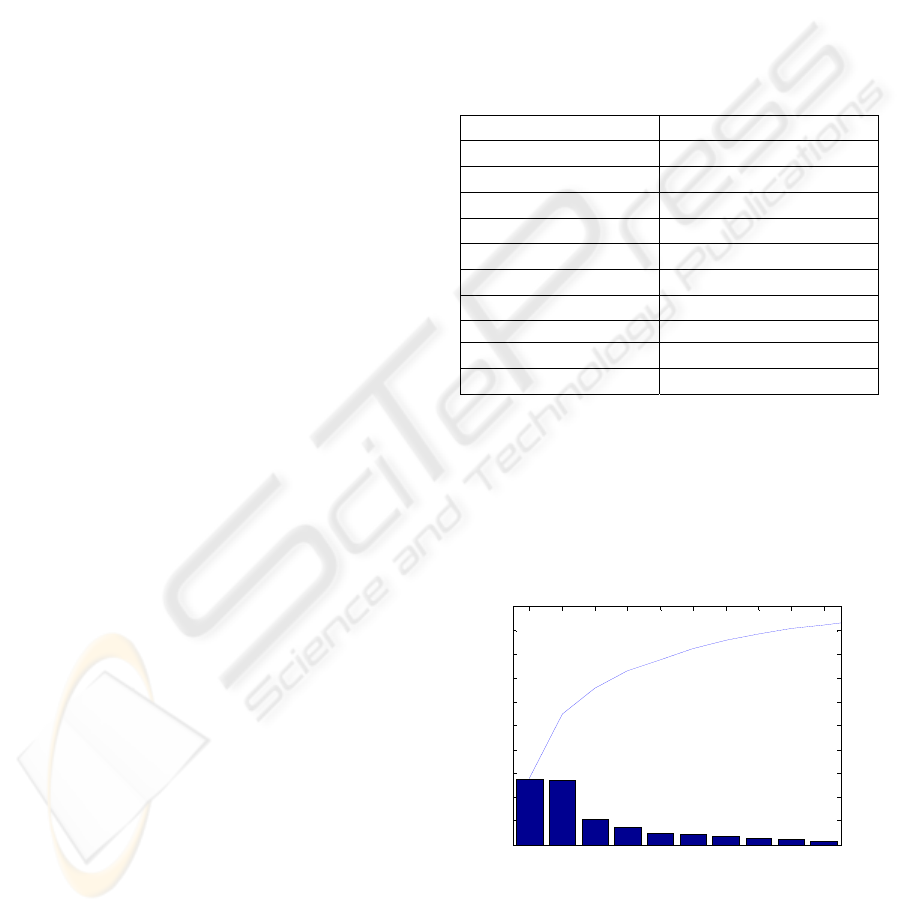
As regards to the PCA, the 32 features were used
to identify the main directions that best represent the
data. Figure
3 shows the amount of information
represented by each component and the cumulated
information given by the first 10 components. It can
be seen that these components enable to represent
93% of the total information in the training set.
1 2 3 4 5 6 7 8 9 10
0
10
20
30
40
50
60
70
80
90
Principal Component
Variance Explained (%)
WISCONSIN 1995 Pronostic : ACP
0%
10%
20%
30%
40%
50%
60%
70%
80%
90%
Figure 3: 10 principal components obtained by ACP and
their power of data representation.
BIOINFORMATICS 2010 - International Conference on Bioinformatics
126

3.1.2 Method and Results
In this study, due to the limited number of relapsed
patients, a Leave-One-Out Cross Validation (LOO
CV) strategy has been performed to estimate the rate
of accuracy. This consists of removing one sample
from the dataset, constructing the predictor only on
the basis of the remaining samples, and then testing
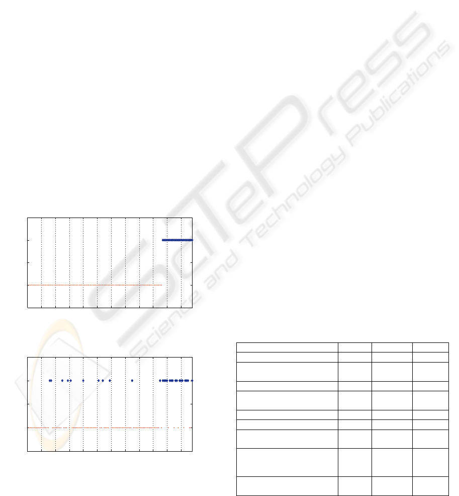
its performance on the removed example. The 118
patients have been ordered: the first 96 have not
relapsed after 24 months and the last 22 relapsed
(ordered in Figure 4 from left to right).
The fuzzy classification results obtained by using
the Gaussian membership function are presented in
Table 2.
A first classification has been performed using
the 32 features and the results are shown in Figure 5.
It can be noted that the overall prognosis is quite
good (85.59%) with a prediction of relapse of
72.73% (which is acceptable given the reduced
amount of relapsed patients in the dataset). In Figure
4 it can be seen that 7 patients (points starting from
patient number 97) who effectively relapsed have
not been well recognized. It is clear that a good
analysis of the results must not only consider the
total recognition score but focus on the false
negatives since these patients will not receive an
appropriate treatment.
0 10 20 30 40 50 60 70 80 90 100 110 118
~Relpase
Relapse
Wisconsin Breast Cancer Recurrence
Patients
classes
Figure 4: Wisconsin Breast Cancer ordered dataset.
0 10 20 30 40 50 60 70 80 90 100 110 118
~Relapse
Relapse
LAMDA results
Patients
classes
Figure 5: LAMDA results with 32 features.
A comparison of these results can be made with
those obtained by Wolberg et al. (Wolberg et al.,
1995) using a variant of MSM (MultiSurface
Method) known as MSM-Tree (MultiSurface Tree
Method): 86.3%. This method uses linear
programming iteratively to place a series of
separating planes of the feature space of the
examples (Wolberg et al., 1995). MSM-T is similar
to other decision tree methods such as CART and
C4.5 but has been shown to be faster and more
accurate on several real-world data sets (Bennett,
1992). Although in the reported studies a T-test
feature selection was performed it was not finally
used to build the classifier. On the contrary all
possible combinations of the 32 features were tested
to determine the best set of features leading to the
best class separation. Only four features were
selected: M texture, W area, W concavity, W fractal
dim. The best obtained result (86%) using this
method is comparable to ours. Moreover it is shown
that the introduction of the tumour size and the
lymph nodes as supplementary features did not
improve the performance (77.40%).
Nevertheless, it
is impossible to go further in the comparison since
the authors did not give the rate of the false
negatives.
Complementary studies with preliminary feature
selection step were performed: T-test, entropy and
PCA. The results are given in Table 2. These results
confirm that the features that correspond to the
morphology of the tumour are directly related to the
prediction of relapse. Nevertheless this information
is not sufficient to obtain a comparable accuracy (the
accuracy of general prediction is less than 75% for
T-test and entropy). These results confirm as stated
by (Wolberg et al., 1995), that this kind of feature
Table 2: WBCP recognition results for the 3 feature
selection methods with/without Tumour size and positive
lymph nodes.
Feature selection Total ~Relapse Relapse
T-Test: 10 features 74.58% 77.09% 63.64%
T-Test: 10 features + tumour
size & lymph nodes
78.81% 82.29% 63.64%
Entropy: 10 features 72.88% 77.08% 54.55%
Entropy: 10 features + tumour
size & lymph nodes
76.27% 81.25% 54.55%
PCA: First 10 components 83.05% 93.75% 36.36%
Nuclei cell 30 features 83.05% 85.42% 72.73%
Nuclei cell 30 features +
tumour size & lymph nodes
85.59% 88.54% 72.73%
MSM-T Results (M texture,
W area, W concavity,
W fractal dim.)
86.3% ~ ~
MSM-T Results + tumour size
& lymph nodes
77.4% ~ ~
PROGNOSIS OF BREAST CANCER BASED ON A FUZZY CLASSIFICATION METHOD
127

selection procedure does not allow identifying the
best class separation. When the tumour size and the
number of infected lymph nodes are added to these
10 selected features, an increase of 4% is achieved
in both cases but it remains under the 86% obtained
with the 32 features. In the case of PCA, the results
given in Table 2 seem better. Nevertheless, even if
the overall rate of prediction is more than 83%, the
prediction of relapse (poor prognosis) is very low
(36.36%).
3.2 Ljubljana Prognosis Dataset
For roughly 30% of the patients who undergo an
operation on breast cancer, the disease reappears
after five years. Regarding this dataset, the aim is to
predict whether patients are likely to relapse, which
may influence the treatment they will receive.
The Ljubljana Prognosis dataset contains a total of
286 patients for whom 201 have not relapsed after
five years and 85 who have relapsed (Clark &
Niblett, 1987). For these patients, 9 features are
available (six qualitative and three interval types):
1. Age: 10-19, 20-29, 30-39, 40-49, 50-59, 60-69,
70-79, 80-89, 90-99
2. Menopause: >40, <40, pre-menopause.
3. tumour size: 0-4, 5-9, 10-14, 15-19, 20-24,
25-29, 30-34, 35-39, 40-44, 45-49, 50-54, 55-59.
4. invaded nodes: 0-2, 3-5, 6-8, 9-11, 12-14, 15-17,
18-20, 21-23, 24-26, 27-29, 30-32, 33-35, 36-39.
5. Ablation ganglia: yes, no.
6. malignancy Degree: I, II, III
7. Breast right, left
8. Quadrant: sup. left, inf. left sup. right, inf. right,
center.
9. Irradiation: yes, no
3.2.1 Methods and Results
A cross-validation (50% training, 50% test) has been
performed to estimate the accuracy of the proposed
methodology. Patients with missing data were
excluded from this analysis (9 patients). The results
are given in Table 3. In order to compare these
results with those cited in earlier works (Clark &
Niblett, 1987), a first study consisted in classifying
Table 3: LAMDA results with Ljubljana dataset.
Feature selection Training Test
Whole original
dataset
91% 89.89%
8 features with
interval grade
91.33% 90%
Without irradiated
patients
93% 92.1%
the 277 patients with 9 features as given in the
original dataset: 6 qualitative features including the
degree of malignancy (feature No. 6 given by
modalities I, II or III) and 3 interval features. A
second study was done by treating the grade data as
intervals (I: [3,5], II: [6,7], III: [8,9]). This allows
expressing the linguistic distance between grades,
such as oncologists do naturally.
Table 4: Ljubljana comparative results.
Method Accuracy
MEPAR-miner 92.8%
LAMDA 90%
Isotonic separation 80%
EXPLORE 76.5%
C4.5 72%
AQR 72%
Assist 86 68%
NaiveBayes 65%
The results obtained by considering the grade
type as an interval show the effectiveness of this
method, which gives an accuracy of 91.33% in
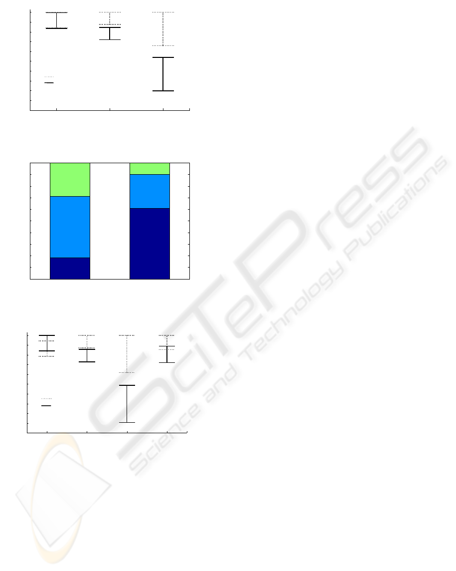
training and 90% in test. Figure 6, 7 and 8 show the
class parameters of interval features obtained in
these two studies. It can be observed that the interval
features “Tumour size” and “Lymph nodes” are
more discriminatory between classes in the two
studies than the “Age” feature. This fact was
established in many previous studies (Deepa et al.,
2005), where it was noted that these two features
still to date are considered as important prognostic
factors. While for the feature “Grade” which makes
the difference between the two studies, even if in the
first study (Figure 7, where it was considered as
qualitative) the difference in the three modalities
frequencies between the two classes can be
observed, the interpretation is still quite ambiguous
since the two classes contains the three grades with a
slight difference. In the second study (Figure 8,
when the grade is considered as interval feature) the
interpretation becomes easier and straightforward.
A third part of the study was to consider only
patients who have not yet undergone an irradiation
treatment (215). This treatment had been applied
systematically to patients with a positive number of
lymph nodes. This implies that the two features:
“irradiation” and the “number of affected lymph
nodes” are correlated with each other. The objective
here is to validate the method precisely to help
physicians on the decision of treatment based on the
results of prognosis beyond 5 years. The results (3rd
line of Table 3) are quite satisfactory, 93% of
accuracy for learning and 92.1% for test. Comparing
these results (Table 4) with those obtained with
BIOINFORMATICS 2010 - International Conference on Bioinformatics
128

Age Tumor size Lymph nodes
0
0.1
0.2
0.3
0.4
0.5
0.6
0.7
0.8
0.9
1
Class interval parameters
interval features
Normalized Intervals
No Recurrence
Recurrence
Figure 6: Classes parameters of interval features (1
st
study).
Recurrence No Recurrence
0
0.1
0.2
0.3
0.4
0.5
0.6
0.7
0.8
0.9
1
Classes
Frequencies
Qualitative grade profile
GRADE 3
GRADE 2
GRADE 1
GRADE 3
GRADE 2
GRADE 1
Figure 7: Classes of the feature “grade” (1
st
study).
Age Tumor size Lymph nodes Grade
0
0.1
0.2
0.3
0.4
0.5
0.6
0.7
0.8
0.9
1
Class interval paramaters
Normalized Intervals
interval features
No Recurrence
Recurrence
Figure 8: Classes parameters of interval features(2
nd
study).
other techniques AQR (Michalski & Larson, 1983),
Assistant (Cestnik et al., 1987), CN2 (Clark &
Niblett, 1989), C4.5 (Quinlan, 1993), Boosters
(Bernhard et al., 2001), Isotonic separation (Ryu et
al., 2007) and EXPLORE (Kors et al., 1997),
LAMDA classification results appear to be as good
as the best results reported previously and gives
comparable results to MEPAR-miner algorithm
(Aydogan et al.) which achieves 92.8% of accuracy.
4 CONCLUSIONS
This study has shown that the fuzzy classification
provides satisfactory results in the prognosis of
breast cancer. Comparing these results with those of
the literature shows that they are either very similar
or higher. The improvement of the quality of these
results is based primarily on the recent development
of a method that handles efficiently interval data as
well as both quantitative and qualitative data; this
property is one of the main features of the LAMDA
method. Although other methods may yield results
that are equal to those obtained with the LAMDA
method, the advantage of using LAMDA is the
significant gain in the interpretation simplicity. This
is particularly useful in the medical context where a
significant insight into the nature of the problem
under investigation is recommended.
Future works will be devoted to develop a
feature selection procedure based on a wrapper
method which consists in using the classification
algorithm itself to evaluate the goodness of a
selected feature subset.
REFERENCES
Aguado J. C., Aguilar-Martin J., 1999. A mixed
qualitative-quantitative self-learning classification
technique applied to diagnosis, QR'99 The Thirteenth
International Workshop on Qualitative Reasoning.
Chris Price, 124-128.
Aguilar J., Lopez De Mantaras R. 1982. The process of
classification and learning the meaning of linguistic
descriptors of concepts. Approximate reasoning in
decision analysis. p. 165-175. North Holland.
Aydogan E.K, Gencer C. 2008. Mining classification rules
with Reduced-MEPAR-miner Algorithm. Applied
Mathematics and computation. 195 p. 786-798.
Bennett K. P., 2001. Decision Tree construction via Linear
Programming. Evans editor. Proceedings of the 4
th
Midwest and Cognitive Science Society Conference.
p,97-101.
Bernhard, P., Geopprey, H.,& Gabis,S., 2001. Wrapping
Boosters against noise. Australian Joint Conference on
Artificial Intelligence.
Billard, L.,
2008. Some analyses of interval data. Journal
of Computing and Information Technology - CIT 16,4.
p.225–233.
Cestnik, B., Kononenko, I.,& Bratko, I., 1987. Assistant-
86: A knowledge elicitation tool for sophisticated
users. Progress in Machine Learning. Sigma Press. p.
31-45. Wilmslow.
Clark, P., Niblett, T., 1987. Induction in Noisy Domains.
Progress in Machine Learning. (from the Proceedings
of the 2
nd
European Working Session on Learning). p.
11-30. Bled, Yugoslavia: Sigma Press.
PROGNOSIS OF BREAST CANCER BASED ON A FUZZY CLASSIFICATION METHOD
129

Clark, P., Niblett, T., 1989. The CN2 Induction algorithm.
Machine Learning 3 (4). p. 261-283.
Deepa, S., Claudine, I., 1987. Utilizing Prognostic and
Predictive Factors in Breast Cancer. Current
Treatment Options in Oncology 2005, 6:147-159.
Current Science Inc.
Holter, R., 1993. Very simple classification rules perform
well on most commonly used datasets. Machine
Learning 11 (1). p. 63-90.
Isaza, C., Kempowsky, T., Aguilar, J., Gauthier, A., 2004.
Qualitative data Classification Using LAMDA and
other Soft-Computer Methods. (Recent Advances in
Artificial Intelligence Research and Development. IOS
Press).
Kira, R., Rendell, L. A., 1992.
A practical approach to
feature selection. Proc. 9
th
International Conference
on Machine Learning. (1992),pp. 249-256.
Kors, J.A., Hoffmann, A.L., 1997. Induction of decision
rules that fulfil user-specified performance
requirements. Pattern Recognition Letters 18 (1997),
1187-1195.
Michalski, R., Larson, J.,
1983. Incremental generation of
VL1 hypotheses: the underlying methodology and the
description of program AQ11. Dept of Computer
Science report (ISG 83-5). Univ. of Illinois. Urbana.
Murphy, P., Aha, D., 1995.
UCI repository of machine
learning databases. Dept. Information and Computer
Science. University of California. Irvine
(http://www.ics.uci.edu/~mlearn/MLRepository.html).
Piera N. and Aguilar J., 1991. Controlling Selectivity in
Non-standard Pattern Recognition Algorithms,
Transactions in Systems, Man and Cybernetics, 21, p.
71-82.
Quinlan, J.,
1993. C4.5: Programs for Machine learning.
Morgan Kaufmann. San Mateo, CA.
Ryu, Y. U., Chandrasekaran, R., Jacob V.S., 2007. Breast
cancer predicition using the isotonic separation
technique. European Journal of Operational
Research, 181. P. 842-854.
Wolberg, W.H., Street, W.N., Mangasarian, O.L., 1995.
Image analysis and machine learning applied to breast
cancer diagnosis and prognosis. Analytical and
Quantitative Cytology and Histology, 17 (2). p. 77-87.
APPENDIX
As it has been described, in the LAMDA approach
the GAD is obtained by using a fuzzy aggregation
function applied to the MADs considered
independently. In the present work the MAD
function used is:
[]
2
1
2
/exp
iik
ik
ik
x
MAD x C
ρ
σ
⎛⎞
⎛⎞
−
⎜⎟
=−
⎜⎟
⎜⎟
⎝⎠
⎝⎠
(A.1)
where the parameters of class C
k
are respectively
the mean
ρ
ik
and the standard deviation σ
ik
of the
elements of this class. Therefore, if the aggregation
function chosen is
Γ , for an object X=[x
1
,...,x
i
,...x
n
]
m
R
∈
, its global membership to class C
k
is
GAD[X/C
k
]=Γ(MAD[x
1
/C
k
],..., MAD[x
i
/C
k
],...
MAD[x
n
/C
k
])
(A.2)
Nevertheless by using the Gaussian type function
it is possible to take into account the correlation
between features in the definition of the GAD, as
follows:
[]
()()
(
)
1
1
2
/exp
T
kkkk
GAD X C X X
ρ
σρ
−
=−− −
(A.3)
where the parameters of class C
k
are ρ
k
and σ
k
,
respectively the mean vector and the covariance
matrix of the elements of this class. To take into
account the features correlation it is proposed a
transformation to calculate the MADs in a new basis
such as they are uncorrelated to each other. This
transformation relies on the following theorem:
Theorem: given a set of vectors
{}
NnX
n
L,1=
, its mean
vector is M (A.4) and its covariance (correlation)
matrix is P (A.5) assumed to be invertible.
1,
1
n
nN
M
X
N
=
=
∑
L
(A.4)
()()
1,
1
1
T
nn
nN
PXMXM
N
=
=−−
−
∑
L
(A.5)
There exists always a linear transformation T
such that the covariance matrix of
nn
TXY =
is
diagonal.
Proof: A square regular matrix P is diagonalizable if
and only if there exists a basis consisting of its
eigenvectors. The matrix B having these basis
vectors as columns is such that
1
R
BPB
−
=
will be
a diagonal matrix. The diagonal entries of this
matrix are the eigenvalues of P. Therefore the
transformation T=B
-1
such that Y
i
=T.X
i
transforms
the mean of the set {Y
n
|n=1,...,N} into:
1,
1
n
nN
K
TX TM
N
=
==
∑
L
(A.6)
and the covariance matrix into:
()()
1
1,
1
1
1
1
T
nn
nN
R
TX M X M T
N
TPT
BPB
−
=
−
−
=−−
−
=
=
∑
L
(A.7)
So that
()()
(
)
()()
1
1
2
1
2
1,
exp
exp
T
nn
T
ni i ni i
im
i
YKRYK
yk yk
r
−
=
−− −
⎛⎞
−−
⎜⎟
=−
⎜⎟
⎝⎠
∏
L
(A.8)
where
.
i
r
is the i
th
eigenvalue of R, and the mean
∑
=
=
Nn
nii
y
N
k
L,1
1
.
By analogy this property is extended further than
the product towards any fuzzy aggregation
function
Γ
.
BIOINFORMATICS 2010 - International Conference on Bioinformatics
130