SEGMENTATION OF SES FOR PROTEIN STRUCTURE

ANALYSIS

Virginio Cantoni, Riccardo Gatti and Luca Lombardi

University of Pavia, dept. of Computer Engineering and Systems Science,Via Ferrata 1, Pavia, Italy

Keywords: Protein structure analysis, Protein-protein interaction, Surface labeling, Convex hull, Distance transform.

Abstract: The morphological complementarities of molecular surfaces provides insights for the identification and

evaluation of binding sites. A quantitative characterization of these sites is an initial step towards protein

based drug design. The final goal of the activity here presented is to provide a method that allows the

identification of sites of possible protein-protein and protein-ligand interaction on the basis of the

geometrical and topological structure of protein surfaces. The goal is to discover complementary regions

(that is with concave and convex segments that match each others) among different molecules. In particular,

we are considering the first step of this process: the segmentation of the protein surface in protuberances and

cavities through an approach based on an analysis of the molecule Convex Hull and on the Distance

Transform.

1 INTRODUCTION

An important research activity, with the large set of

proteins in the current Protein Data Bank (PDB), is

the prediction of interactions of these molecules by

the discovery of similar or of complementary

regions on their surfaces. When a novel protein with

unknown functionalities is discovered,

bioinformatics tools are used to screen huge datasets

of proteins searching for candidates binding sites.

More specifically, if a surface region of the novel

protein is similar to that of the active site of another

protein with known function, the function of the

former protein can be inferred and also its molecular

interaction can be predicted. Active sites are

generally in concave and deep spots of the surface

that are called “pockets”.

Much work has been done on the identification

and the analysis of the binding sites of proteins using

various approaches based on different protein

surface descriptions and matching strategies. The

techniques employed are ranging from geometric

hashing of triangles of points and their associated

physico-chemical properties (Shulman, 2004), to

clustering based on a representation of surfaces in

terms of spherical harmonic coefficients (Glaser,

2006) or by a collection of spin-images (Bock, 2007

– Bock, 2008) or by context shapes (Frome, 2004),

to clique detection on the vertices of the triangulated

solvent-accessible-surface (SAS) (Akatsu, 1996), to

local surface ‘buriedness’ evaluation (Brady, 2000).

The goal of this work is to segment the protein

surface in protuberances and cavities. This

segmentation is based on the Distance Transform

(DT) applied to the volume obtained subtracting the

molecule to the its Convex Hull (CH). Once

obtained protrusions and inlets, for each segment, a

few features are provided including area and volume

of the inlet, area and circumference of the pocked

mouth opening, curvature (Cantoni, 2009) and travel

depth. These features are the basic parameters for

the first screening of compatible sites. A more

precise subsequent experimental analysis on a

limited subset of cases must be then applied.

This paper is organized as follows: section two

shows a survey of approaches for segmentation and

analysis of protein surfaces through the convex hull;

in section three is introduced the solution proposed,

then in section four a few results on artificial test-

images and on true proteins molecules are presented.

The final section, section five, provides a few

concluding remarks and briefly describes our

planned activity in the near future.

Cantoni V., Gatti R. and Lombardi L. (2010).

SEGMENTATION OF SES FOR PROTEIN STRUCTURE ANALYSIS.

In Proceedings of the First International Conference on Bioinformatics, pages 83-89

DOI: 10.5220/0002590900830089

 SciTePress

2 SURFACE ANALYSIS

SEGMENTATION THROUGH

THE CONVEX HULL

The CH of a molecule is the smallest convex

polyhedron that contains the molecule points. In R

the CH is constituted by a set of facets, that are

triangles, and a set of ridges (boundary elements)

that are edges. A practical O(n log n) algorithm for

general dimensions CH computing, is Quickhull

(Barber, 1996), that uses less space and executes

faster than most of the other algorithms.

The CH approach for molecular segmentation is

not new. The first paper applying this method, to

authors’ knowledge, is (Meier, 1995). The Quickhull

algorithm, is applied to the SAS which is defined by

the center of a water-sized probe sphere (usually

with radius values ranging between 1.4 and 1.8 Å)

‘rolling over the van der Waals surface of the atom’.

The technique is based on two specificities: i) the

tips lie directly on the CH surface: they are the

common points between molecule and CH surfaces;

ii) inlets and holes are ‘normally’ covered by large

facets of the CH surface. Both specificities are not

necessary conditions (the second is even not

sufficient) to establish the existence of true tips and

inlets: it is just a reasonable first hypothesis.

Moreover, the technique for tip segmentation is

based on a heuristic approach: each tip is extended

on the outside facet for a distance determined by a

global parameter.

Two other different approaches based on the CH

of the atoms centers have been proposed

Edelsbrunner (Edelsbrummer, 1998) and Xie (Xie,

2007). Both apply the Dealunay triangulation

technique, that in 3D have complex counterparts (3D

tetrahedrons), to evaluate quantitatively some

parameters.

The former, through a dual complex (alpha shape)

analysis, provides a quantitative description of the

microenvironments for protein structure based

design. In particular, volume and area of pockets,

area and circumferences of mouth opening, are

evaluated. For the pockets identification, it is used

the discrete flow method, that is the presence of

Delaunay’s tetrahedra disjointed to the dual

complex. In particular, for segmentation purposes,

some geometrical and topological rules allow the

discrimination between two neighboring tetrahedra,

satisfying the previous constraint. Note that, not all

the inlets are identified as pocket (the one for which

the discrete-flow pours to the outside of the CH).

The latter approach is based on a simplified

description that requires only the Cα atoms to

represent the protein structure in order to speed-up

the computation (making the new representation

“scalable to a large data set … yet robust enough to

handle the intrinsic properties of protein

flexibility”). Moreover, the notion of geometric

potential is introduced: this figure quantitatively

describes the microenvironment on the basis of two

heuristic parameters and allows a fast and effective

discrimination for active sites.

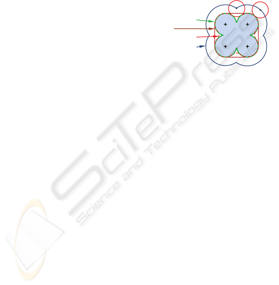
Figure 1: Common 2D representations of surface models

for protein’s molecules: i) in green the van der Waals

surface, directly produced from the atom’s locations

through the van der Waals radii; ii) in red the Solvent-

Excluded Surface SES (also known as the molecular

surface or Connolly surface) generated by the envelope of

a rolling sphere over the van der Waals surface (The

radius of the solvent sphere is usually set to the

approximate radius of a water molecule having a van der

Waals radius of 1.4 Å); iii) in blue the solvent accessible

surface (sometimes called the Lee-Richards molecular

surface) generated by the center of the solvent sphere

rolling over the van der Waals surface; iv) in brown the

convex hull, that coincides also with the SES having a

sphere with an infinite radius.

The CH is also the reference surface for the

molecules analysis based on the ‘travel depth’. The

travel depth parameter (Coleman, 2006 – Giard,

2008), with reference to the SES (see figure 1), is

defined as the shortest path accessible for a solvent

molecule between the protein convex hull and a

given point that belongs to the ‘active’ region of

interest (ROI) delimited by CH and SES. It

represents the physical distance that a ‘sufficiently’

small molecule has to travel to approach a surface

position (the pockets bottom are usually the points

of interest). It is particular the case of tunnels, i.e.

when pockets have no ‘bottom’, in which the

molecule can travel through the entire protein and

the travel depth is delimited by two points belonging

to the CH. In particular (Coleman, 2006) introduced

a technique for computing the travel depth on the

basis of a peculiar distance transform

implementation in the ROI defined above. The

Convex hull

Van der Waals surface

Solvent accessibile

Solvent-excluded

BIOINFORMATICS 2010 - International Conference on Bioinformatics

implementation proposed by Giard et al. has the goal

of speed-up the travel depth computation through a

surface-based propagation algorithm that should be

in general faster than the volume-based DT.

3 TUNNELS AND POCKETS

DETECTION

In the discrete space the protein and the CH are

defined in a cubic grid V of dimension L x M x N

voxels. Note that the grid is extended one voxel

beyond the minimum and maximum coordinate of

the SES in each orthogonal direction (in this way

both SES and CH borders are inside the V border).

The voxel resolution adopted is 0.25 Å, so as to be

small enough to ensure that, with the used radii in

biomolecules atoms, any concave depression or

convex protrusion is represented by at least one

voxel.

Let us call R the region between the CH and the

SES (the concavity volume (Borgefors, 1996)), that

is:





(1)

Let us call B

the set border voxels of CH, that is:











(2)

Whererepresent the erosion operator of

mathematical morphology and K the discrete

unitarian sphere (in the discrete space a 3x3x3

cube!).

Within the region R the following propagation is

applied:

















A = B

;

N = (A ⊕ K)∩R;

E = N – A;

while E ≠ ∅ do

























;

A = N;

N = (A ⊕ K)∩R;

E = N – A;

done

where:

i. A represents the increasing set of voxels

contained in R;

ii. E corresponds to the recruited set of near

neighbors of A contained in R (i.e. the voxels

reached by the last propagation step);

iii. 



















represents the

minimum value among the distances 



in

the near neighbors belonging to D already

defined, incremented by the displacement





between the locations (e, n): that is, if e

and n have a common face 



; if e and

n have a common edge 







; if e and n

have a common vertex 







. In three

dimensions, the total number of the near

neighbor elements of p is 26: six of them

that share one face and have distance equal

to 1 from the voxel p, twelve neighbors that

share only an edge and are at distance







and eight that share only a vertex and are at

distance





always from voxel p. At each

iteration, new voxels, inside R, are reached

by the propagation process and the value

they take is determined by the neighbor

distance (from the convex hull) and the

voxels distance from the neighbor involved;

this in order to simulate an isotropic

propagation process and the proper distance

evaluation.

iv. E = ∅ corresponds to the regime

condition: no other changes are given and

the connected component of R, adjacent to

the border B

is completely covered.

The values in D represent the distance of each voxel

of A from the border of B

and A corresponds to

the connected component of R adjacent to the

border.

Having A, it is possible to easily identify and

eventually remove the cavities C, that are the

volumes completely enclosed in the macromolecule

C = CH - A - M (3)

Figure 2a: A 2D example for tunnels and pockets

detection composed of three connected components (in

brown). The closed curve in black corresponds to the

convex hull, and the border BCH in gray embodies the

area under analysis and is the starting set of voxels for the

propagation process.

SEGMENTATION OF SES FOR PROTEIN STRUCTURE ANALYSIS

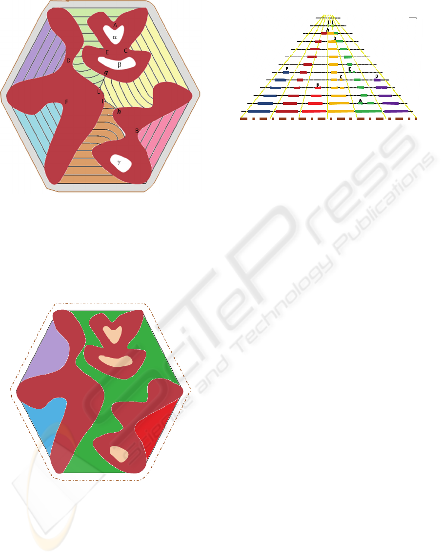
Figure 2b: Results achieved after the propagation phase.

Three pockets are identified, in blue, red and violet

respectively. For the other three sides the propagation

process converges: firstly there is the merging of the

green and yellow waves, then the yellow and brown

waves, and the complete coverage of the accessible areas

is achieved in location L and I respectively. Note the three

internal inaccessible components, in white, with labels

α, β, γ.

Figure 2c: Final segmentation, showing the tunnel (in

green) and the three detected pockets.

Figure 2d: Another representation of the results after the

propagation phase. The letters B, D, F correspond to the

top of three pockets (see also figure 2b)). The letters A, C,

and E correspond to three local tops that are adjacent to

important inlets. The letters g and h corresponds to

convergences towards the tops I and L which identify a

threelobate tunnel.

In order to separate the different pockets and

tunnels the volume A must be partitioned into a set

of disjoint segments P

SES

= {P

, … , P

where N is the number of inlets. The partition must

satisfy the following condition:

∩ P

∅

, i ≠ j

(4)

∪ ·· · ∪ P

= A

(5)

As can be easily extended form the 2D example

of Figure 2, starting from the total set of convex hull

facets, several waves are generated and propagation

proceeds up to the complete coverage of the volume

A: the connected component of R adjacent to the

border. During the propagation phase two sets of

salient points are identified: local tops LT

(represented by capital letters in Figure 2) and wave

convergence WC points (lower case).

The LT set is exploited for the segmentation process.

The cardinality of LT corresponds to N

max

the

maximum number of segments/inlets that can be

considered. The effective number of segments, that

determines obviously the number and the

morphology of pockets and tunnels, is found out on

the basis of two heuristic parameters: i) the

minimum travel depth value of the local tops TD

;

ii) an evaluation of near neighbor pivoting effects

PEs. The threshold TD

is introduced because the

surface’s irregularities and the digitalization process

produce small irrelevant spurious cavities. The

thresholds PEs take into account morphological

aspects insight important cavities and can be

characterized by two different features: the nearness

of others, more significant, local tops (τ

) and the

BIOINFORMATICS 2010 - International Conference on Bioinformatics

relative values of the local-top travel-distance (τ

). in

general faster than the volume-based DT.

4 IMPLEMENTATION AND

RESULTS

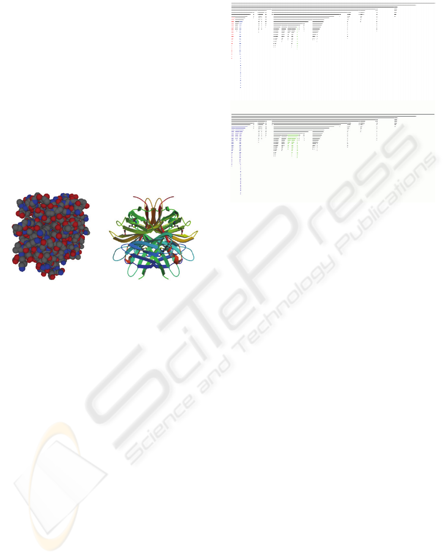
We start from the ‘space-filling’ representation of

the protein, where atoms are represented as spheres

with their van der Waals radii (this representation is

directly derived from PDB files which supply the

ordered sequence of 3D positions of each atom’s

center). Figure 3 shows the image produced by our

package for Apostreptavidin Wildtype Core-

Streptavidin with Biotin structure (1MK5 in PDB).

Figure 3: On the left the ‘space filling’ representation of

1MK5. The colors follow the standard CPK scheme. On

the right the correspondent secondary structure

representation.

A first critical decision is the space resolution level

for the analysis. The results presented here are given

with a resolution of 0.25 Å, which entails a van der

Waals radius of more than five voxels to the smallest

represented atoms. The algorithm is then applied to

the SES obtained from the quoted surface, after the

execution of a closure operator using a sphere with

radius of 1.4 Å , about 6 voxels, (corresponding to

the conventional size of a water molecule) as

structural element. It is worth to point out that this

closure operation excludes possible passage through

apertures with a section of less than 6.15 Å

(about

99 voxels). Note that, as it has been mentioned in

section 3, the grid is extended one voxel beyond the

minimum and maximum coordinate of the SES in

each orthogonal direction (in this way both SES and

CH borders are inside the V border).

Two other parameters characterize the execution:

the minimum passage section θ

(obviously

≥100); the maximum mouth aperture θ

. The

former has been fixed on a heuristic base to 150

Voxels (which for a circle corresponds to a radius of

7 voxels). The latter has been applied with two

different values: 2000, 7500.

Figure 4: A representation of the results after two

segmentation phases with θ

equal to 2000 and 7500 in a)

and b) respectively. Note that no tunnel is present, and 9

pockets have been identified and differently colored. In

particular the first three pockets in the top figure are then

represented in figures 5, 6 and 7 corresponding to θ

=2000

and the first two pockets in figures 8 and 9 having

=7500.

In Figure 4 the results of the segmentation

process are given. This process is executed in two

phase: in the onward propagation the set of the

pocket’s local top is identified; later a backward

parallel propagation from each of the tops with

identify all the pockets is executed. Finally, it is

applied the near neighbor pivoting process, which

(with τ

=10 and τ

=5) leads to the final result

shown. Figures 5-9 show the pockets with the

highest travel distance (obviously the parameters of

reference can be one of the others features – e.g. the

pocket volume -, or even a combination of features –

e.g. travel distance and pocket volume-) for different

values of the parameter θ

. Each pocket is

represented with a lateral and frontal view

(respectively on the left and on the right side of each

figure).

As it can seen from figure 4, having θ

=150 voxels

no tunnels are present, but there are several well

characterized pockets which can be easily

characterized and evaluated. In particular the

dependence of the results of the segmentation

process from the different parameters is pointed out.

The algorithms has been tested on a 2.20 GHz x86

Intel processor the computing time is about 12

seconds for the protein 1MK5 with 127 residues and

1844 atoms.

SEGMENTATION OF SES FOR PROTEIN STRUCTURE ANALYSIS

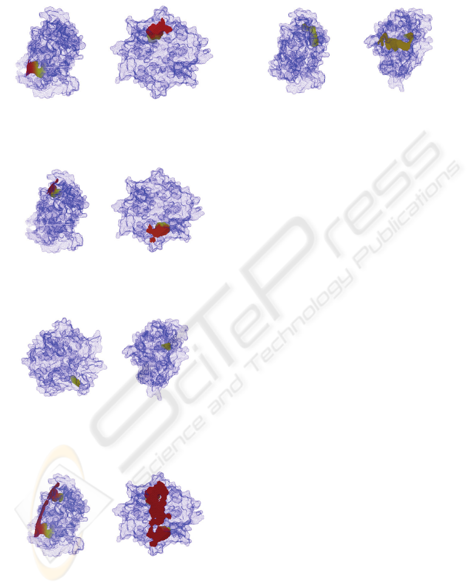
Figure 5: The pocket with the highest travel depth (highest

distant from the CH): 57, with the control parameter θ

the value: 2000. Note that the red component testifies that

the ‘pocket mouth’ is close to the CH.

Figure 6: The pocket with the second highest travel depth:

35, with θ

= 2000. Note that also in this case, the ‘pocket

mouth’ is close to the CH.

Figure 7: The pocket with the third highest travel depth:

34, with θ

= 2000. Note the absence of the red

component: the ‘pocket mouth’ is at a distance of 20

voxels from the CH.

Figure 8: The pocket with the highest travel depth

achieved with θ

= 7500. Note that for this value of the

control parameter the two highest pocket achieved with θ

= 2000 are fused together realizing a large ‘pocket mouth’

more close to the CH.

Figure 9: The pocket with the second highest travel depth

with θ

= 7500. Note that this is the evolution of the

previous third pocket and is characterized by a large

‘pocket mouth’ and the presence of the red component

(that is the mouth is closer to the CH).

5 CONCLUSIONS

The final goal of the activity here presented is to

provide a method that allows the identification of

sites of possible protein-protein and protein-ligand

interaction on the basis of the geometrical and

topological structure of protein surfaces. The goal is

then to discover complementary regions (that is with

concave and convex segments that match each

others) among different proteins. In particular, we

are considering the first step of this process: the

segmentation of the protein surface in various

pockets and tunnels. The next step of our activity is

related to the characterization of each of the

extracted segment through morphological and

topological quantitative descriptors (including travel

depth, mouth aperture, curvature, volume) that can

be combined with the local biochemical features

(types of residues and their characteristics) to detect

and specialize the active sites of a protein.

REFERENCES

Akutsu T, 1996. Protein structure alignment using

dynamic programming and iterative improvement. In

IEICE Trans. Inf. and Syst., Vol. E78-D, pp. 1-8.

Barber CB, Dobkin DP, and Huhdanpaa H, 1996. The

Quickhull Algorithm for Convex Hull. In ACM

Transactions on Mathematical Software, Vol. 22, N. 4,

pp. 469-483.

Bock ME, Garutti C, Guerra C, 2007. Spin image profile:

a geometric descriptor for identifying and matching

protein cavities. In Proc. of CSB, San Diego.

Bock ME, Garutti C, Guerra, C, 2008. Cavity detection

and matching for binding site recognition.

In Theoretical Computer Science,

doi:10.1016/j.tcs.2008.08.018.

Borgefors G and Sanniti di Baja G, 1996. Analyzing

BIOINFORMATICS 2010 - International Conference on Bioinformatics

Nonconvex 2D and 3D Patterns. In Computer Vision

and image Understanding, vol. 63, N. 1, pp. 145-157.

Brady GP, Stouten PFW, 2000. Fast prediction and

visualization of protein binding pockets with PASS. In

J Comput-Aided Mol Des, 14, pp. 383-401.

Cantoni V, Gatti R, and Lombardi L, 2009. Towards

Protein Interaction Analysis through Surface

Labeling. ICIAP 2009, in press.

Coleman RG, Sharp KA, 2006. Travel Depth, a New

Shape Descriptor for Macromolecules: Application to

Ligand Binding. In J. Mol. Biol., Vol. 362, pp. 441-

458. 1MK5 1A0Q 1ATJ PDBbind, 29 di pg 451,

1H2R

Edelsbrunner H, Liang J and Woodward C, 1998.

Anatomy of protein pockets and cavities: measurement

of binding site geometry and implications for ligand

design. In protein Science 7, pp. 1884-1897.

Frome A, Huber D, Kolluri R, Baulow T and Malik J,

2004. Recognizing Objects in Range Data Using

Regional Point Descriptors. In Computer Vision -

ECCV, pp. 224-237.

Giard J, Rondao Alface Patrice, Macq B, 2008. Fast and

accurate travel depth estimation for protein active site

prediction. In SPIE Electronic Imaging 2008, San

Jose, California USA, San Jose Célifornia, USA,

6812, pp. 0Q-10Q.

Glaser F, Morris RJ, Najmanovich RJ, Laskowski RA and

Thornton JM, 2006. A Method for Localizing Ligand

Binding Pockets in Protein Structures. In PROTEINS:

Structure, Function, and Bioinformatics, 62, pp. 479-

488.

Meier R, Ackermann F, Hermann G, Posch S, and Sagerer

G, 1995. Segmentation of molecular surfaces based on

their convex hull. In Proceedings IEEE International

Conference on Image Processing, pp. 552-554. 2utg

Shulman-Peleg A, Nussinov R and Wolfson H, 2004.

Recognition of Functional Sites in Protein Structures.

In J. Mol. Biol., 339, pp. 607-633.

Xie L and Bourne PE, 2007. A robust and efficient

algorithm for the shape description of protein

structures and its application in predicting ligand

binding sites. In BMC Bioinformatics, 8 (Suppl 4):S9.

SEGMENTATION OF SES FOR PROTEIN STRUCTURE ANALYSIS