ARTIFICIAL NEURAL NETWORKS LEARNING IN ROC SPACE
Cristiano Leite Castro
Federal University of Lavras, Department of Computer Science
Campus Universit´ario - Caixa Postal 3037, 37200-000, Lavras, Brazil
Antˆonio Padua Braga
Federal University of Minas Gerais, Department of Electronics Engineering
Av. Antˆonio Carlos, 6.627 - Pampulha, 30161-970, Belo Horizonte, Brazil
Keywords:
Multi-Layer Perceptron (MLP), Backpropagation algorithm, ROC analysis, Imbalanced data sets, Cost-
sensitive learning.
Abstract:
In order to control the trade-off between sensitivity and specificity of MLP binary classifiers, we extended
the Backpropagation algorithm, in batch mode, to incorporate different misclassification costs via separation
of the global mean squared error between positive and negative classes. By achieving different solutions
in ROC space, our algorithm improved the MLP classifier performance on imbalanced training sets. In our
experiments, standard MLP and SVM algorithms were compared to our solution using real world imbalanced
applications. The results demonstrated the efficiency of our approach to increase the number of correct positive
classifications and improve the balance between sensitivity and specificity.
1 INTRODUCTION
Binary classifiers based on Artificial Neural Networks
(ANNs) have two objectives related to the perfor-
mance of each class: one describes the classification
accuracy for abnormal or positive examples (sensi-
tivity) whereas the other describes the accuracy for
normal or negative examples (specificity). In gen-
eral, the simultaneous maximization of both objec-
tives is achieved indirectly, through minimization of a
cost function based on global training set error, such
as, the mean squared error (Haykin, 1994). This is
the case of many learning algorithms designed for the
Multi-Layer Perceptron (MLP) topology since the in-
troduction of the standard Backpropagationalgorithm
(Rumelhart and McClelland, 1986). However, it is
well explored in the literature that, when the global
error is minimized, the balance between sensitivity
and specificity is affected by the difference between
the class prior distributions (Provost et al., 1998),
(Provost and Fawcett, 2001) and (Cortes and Mohri,
2004).
When training sets are imbalanced, classifiers usu-
ally present a good performance for the majority class
but their performance for the minority class is poor.
This occurs mostly because the global training er-
ror considers different errors as equally important as-
suming that the class prior distributions are relatively
balanced (Provost and Fawcett, 2001). In addition,
according to (Elkan, 2001), the majority class natu-
rally imposes higher misclassification costs invalidat-
ing the uniform cost assumption made by the global
error. Considering the case of most real world prob-
lems, when the class imbalanced ratio is huge, (Wu
and Chang, 2005) observed that the separation sur-
face learned by ANNs is skewed toward the minority
class. Consequently, test examples belonging to the
small class are more often misclassified than those be-
longing to the prevalent class.
To overcome this problem, different methods have
been proposed. One approach is based on the data
preprocessing in input space in order to balance the
class distributions (for a good review of these meth-
ods see, for instance, (Weiss, 2004)). In the context
of ANNs, (Japkowicz, 2000) evaluated resampling
techniques in MLP classifiers and concluded that they
were effective. Similarly, (Zhou and Liu, 2006) in-
vestigated the use of undersampling, oversampling,
threshold-moving and ensemble models for the devel-
opment of cost sensitive ANNs. Recently, in (Sun
484
Leite Castro C. and Padua Braga A. (2009).
ARTIFICIAL NEURAL NETWORKS LEARNING IN ROC SPACE.
In Proceedings of the International Joint Conference on Computational Intelligence, pages 484-489
DOI: 10.5220/0002324404840489
Copyright
c
 SciTePress

et al., 2007), the authors compared several cost sensi-
tive boosting algorithms to address the learning prob-
lem with imbalanced data sets. The main criticism of
the data preprocessing approach is the violation of the
randomness assumption of the sample (training set)
drawn from the target population. From a statistical
point of view, as long as the sample is drawn ran-
domly, it can be used to estimate the population dis-
tribution. Once the sample distribution is changed, by
using resampling techniques, it can no longer be con-
sidered random. Nevertheless, these strategies have
presented better results than the original methodol-
ogy.
In the other approach, learning algorithms are
adapted to improve performance of the minority class.
In particular, in the case of ANNs, most of these
strategies are based on the cost function modifica-
tions. In (Kupinski and Anastasio, 1999), (Sanchez
et al., 2005), (Everson and Fieldsend, 2006) and
(Graening et al., 2006), for instance, multi-objective
genetic algorithms (MOGA) have been proposed to
directly optimize sensitivity and specificity. In this
case, these algorithms produce a set of non-dominated
solutions describing the trade-off between these two
measures (pareto set). The drawbacks of the multi-
objective evolutionary algorithms are the high pro-
cessing time and the difficulty in setting the param-
eters. Moreover, a decision algorithm is necessary
to select the solution (operation point) in the pareto
set. In the works mentioned earlier, the authors ob-
served that the choice criterion is quite dependent on
the problem to be solved.
The algorithm proposed in this paper is also based
on the cost function modification. Using MLP bi-
nary classifiers, we extended the standard Backprop-
agation algorithm (in batch mode) to incorporate dif-
ferent missclassification costs via separation of the
global mean squared error between the positive and
negative classes. The objective is to control the
trade-off between sensitivity and specificity achiev-
ing different solutions in ROC space. Our experi-
mental results on both synthetic and real world data
sets (from UCI Repository (Asuncion and Newman,
2007)) show that our modified Backpropagation al-
gorithm is effective to obtain robust solutions for im-
balanced problems.
2 ROC SPACE
According to ROC Analysis (Egan, 1975), the perfor-
mance of some binary classifier on a particular data
set may be summarized by a confusion matrix (see
Table 1) (Fawcett, 2004). Each entry E
kj
of the confu-
sion matrix gives the number of the examples, whose
true class was C
k
and that were actually classified as
C
j
. Hence, the entries along the major diagonal repre-
sent the correct decisions made: number of true pos-
itives (TP) and true negatives (TN); and the entries
off this diagonal represent the errors: number of false
negatives (FN) and false positives (FP).
Table 1: Confusion Matrix.
predicted pos predicted neg
actual pos TP FN
actual neg FP TN
From this matrix, the metrics sensitivity (true pos-
itive rate) and specificity (true negativerate) can be es-
timated by the Equations 1 e 2, respectively. The ROC
Space is defined as a graph which plots the true posi-
tive rate (sensitivity) as a function of the false positive
rate (1− specificity) (Fawcett, 2004). After evaluating
a data set, each classifier produces a pair (sensitivity,
1− specificity) correspondingto a single point in ROC
space.
sensitivity =
TP
TP + FN
(1)
specificity =
TN
TN + FP
(2)
3 MODIFIED
BACKPROPAGATION
ALGORITHM
In this Section, we describe our method to control the
trade-off between sensitivity and specificity of Multi-
Layer Perceptron (MLP) binary classifiers. The ba-
sic idea behind it is the separation of the global mean
squared error and its gradient vector between the posi-
tive and negative classes. The theoretical foundations
are based on the formulation of the standard Back-
propagation algorithm (Rumelhart and McClelland,
1986) in batch mode, where the weights are updated
only after all examples have been presented once for
the network.
3.1 MLP Neural Network
Our approach considers Multi-Layer Percetron (MLP)
neural networks with d inputs, one hidden layer with
h nodes (units) and one output layer containing a sin-
gle node, as shown in Figure 1.
ARTIFICIAL NEURAL NETWORKS LEARNING IN ROC SPACE
485

Figure 1: Multi-Layer Perceptron neural network topology
considered in this work.
The activation of each hidden node j, due to the
presentation of an input example (signal) x, is given
by,
y
j
= f (u
j
) = f
d
∑
i=0
x
i
w
ji
!
. (3)
where each w
ji
corresponds to a weight between the
hidden node j and the input unit i. Similarly, the ac-
tivation of the output node is based on the outputs of
the hidden nodes,
z = f (v) = f
h
∑
j=0
y
j
w
j
!
. (4)
where each w
j
represents a weight between the output
node and the hidden unit j. For the sake of simplicity,
the bias was considered as an extra (input/hidden)unit
whose value is equal to 1.
Since the scope of the method is limited to binary
classification problems, we considered only one sin-
gle output node and use sigmoid activation functions
(hyperbolic tangent) f(·) for all nodes of the network.
Thus, the classification of a given example x is based
on the signal of the output z.
Consider also a training set T =
{(x
1
, t
1
), ·· ·(x
p
, t
p
), ·· ·(x
n
, t
n
)} containing n ex-
amples. The error obtained in the output node due
to the presentation of the p-th training example is
defined as follows,
ε
(p)
(w) =
1
2

t
(p)
− z
(p)

2
(5)
where z
(p)
and t
(p)
correspond to the output and target
values for the example p, respectively. The vector w
denotes the collection of all weights of the network.
From the definition of the error for the p-th training
example, the cost function mean squared error can be
calculated according to the following equation,
E(w) =
1
n
n
∑
p=1
ε
(p)
(w) (6)
3.2 Global Mean Square Error
Separation
The training set T can be redefined as T = T
+
∪ T
−
,
where T
k
=

(x
k
1
, t
k
1
), ·· ·(x
k
p
, t
k
p
), ·· · , (x
k
n
k
, t
k
n
k
)

, for
k = {+, −}. The vector x
k
p
corresponds to the p-th
example of the class C
k
. The target value for a posi-
tive example x
+
p
is always t
+
p
= +1. The number of
positive examples is given by n
+
. Equivalent defini-
tions hold for the negative class.
Given the data sets T
+
and T
−
, we can describe
the functional E(w) as the sum of the cost functions
E
+
(w) and E
−
(w) which represent the mean square
error for each class,
E(w) = E
+
(w) + E
−
(w) (7)
where E
k
(w) is given by,
E
k
(w) =
1
n
k
n
k
∑
p=1
ε
(p,k)
(w) for k = { +, −} (8)
3.3 Gradient Vectors
From the separation of the functional E(w) in E
+
(w)
and E
−
(w), we can calculate the gradient vector for
each cost function E
k
(w), using the following equa-
tion,
∇E
k
(w) =
n
k
∑
p=1
∂ε
(p,k)
∂w
for k = {+, −} (9)
where
∂ε
(p,k)
∂w
is the gradient vector over all weights of
the network w, calculated due to the p-th example of
the class C
k
.
Each component of the vector
∂ε
(p,k)
∂w
corresponds
to a scalar gradient calculated for a given weight of
the network. These values are estimated using the ba-
sic formulation established in the standard Backprop-
agation algorithm and proposed by (Rumelhart and
McClelland, 1986):
1. for each weight w
j
of the output layer, the scalar
gradient due to p-th example of the class C
k
is
obtained using the following chain rule,
∂ε
(p,k)
∂w
j
=
∂ε
(p,k)
∂z
(p,k)
∂z
(p,k)
∂v
(p,k)
∂v
(p,k)
∂w
j
(10)
IJCCI 2009 - International Joint Conference on Computational Intelligence
486

∂ε
(p,k)
∂w
j
= −

t
(p,k)
− z
(p,k)

f
′

v
(p,k)

y
(p,k)
j
(11)
2. Similarly, the scalar gradient for each weight w
ji
of the hidden layer is given by,
∂ε
(p,k)
∂w
ji
=
∂ε
(p,k)
∂y
(p,k)
j
∂y
(p,k)
j
∂u
(p,k)
j
∂u
(p,k)
j
∂w
ji
(12)
∂ε
(p,k)
∂w
ji
= −

t
(p,k)
− z
(p,k)

f
′

v
(p,k)

w
j
f
′

u
(p,k)
j

x
(p,k)
i
(13)
3.4 Weight Update
The weight update of the standard Backpropagation
algorithm (in batch mode) at iteration (epoch) m, is
defined as follows,
w
(m+1)
= w
(m)
− η∇E

w
(m)

(14)
where w
(m)
is the weight vector at iteration m and η is
a positive constant (learning rate). The update of w
(m)
occurs in opposite direction of the gradient vector.
From the global mean squared error separation,
we can describe the gradient vector ∇E(w) as a
weighted sum of the gradient vectors of E
+
(w) and
E
−
(w),
∇E(w) =
1
λ
+
∇E
+
(w) +
1
λ
−
∇E
−
(w) (15)
where the parameters λ
+
and λ
−
with values vary-
ing from 1 to ∞, are used to constrain (penalize) the
gradient vector magnitudes for the positive and neg-
ative classes, respectively. These parameters are in-
troduced to assign different misclassification costs for
each class and, therefore, to control the trade-off be-
tween sensitivity and specificity of the solutions dur-
ing the learning process.
Note that, when λ
+
and λ
−
assume values equal to
1, the weight update equation from the gradient vec-
tor ∇E(w) leads to the standard solution which min-
imizes the global training error. Otherwise, we can
try to find solutions in different areas of ROC Space
(sensitivity x 1− specificity) according to λ
+
and λ
−
.
4 EXPERIMENTS AND RESULTS
In this Section, we conducted experiments that illus-
trate our approach. Using a two-dimensional syn-
thetic data set, we show that it is possible to control
the MLP learning, obtaining different separation sur-
faces in input space. Moreover, in order to improve
the MLP classifier performance on real world imbal-
anced problems, the parameters λ
+
and λ
−
were ad-
justed to balance the costs imposed by the difference
between the number of class examples.
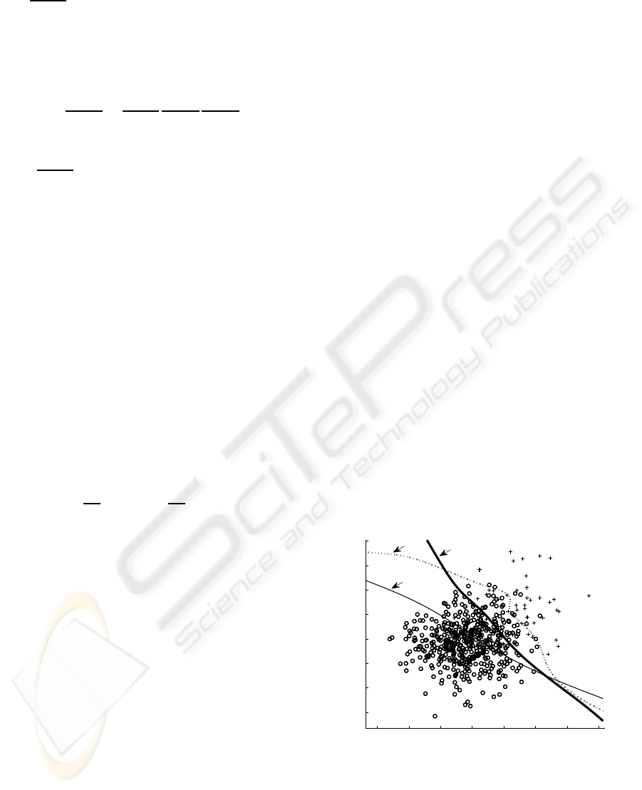
4.1 Synthetic Data
This experiment illustrates the effect caused by the
parameters λ
+
and λ
−
in the separation surfaces
learned by a MLP classifier (topology 2:5:1). A train-
ing set was generated from two-dimensionalGaussian
distributions with mean vectors [0, 0]
T
and [2, 2]
T
and
covariance matrices corresponding to the identity ma-
trix. The ratio between the number of negative (cir-
cles) and positive (plus) examples is 10 : 1.
Figure 2 shows the separation surfaces obtained in
three different situations:
1. Standard solution (dotted line) which minimizes
the global error with λ
+
and λ
−
equal to 1. Per-
formance on the training set ⇒ sensitivity = 0.58
and specificity = 0.98.
2. Solution (bold solid line) which aims to achieve a
balance between the sensitivity and the specificity
with λ
+
= n
+
and λ
−
= n
−
. Performance on the
training set ⇒ sensitivity = 0.90 and specificity =
0.89.
3. Solution (solid line) with high sensitivity by set-
ting the parameters λ
+
= 1 and λ
−
= 100. Perfor-
mance on the training set ⇒ sensitivity = 1.00 and
specificity = 0.68.
−3 −2 −1 0 1 2 3 4
−3
−2
−1
0
1
2
3
4
X1
X2
Sol. 1
Sol. 3
Sol. 2
Figure 2: The effect caused by parameters λ
+
and λ
−
in the
separation surfaces learned by a MLP classifier with topol-
ogy 2:5:1.
The analysis of these results, led to the following
conclusions: the bad performance of the standard so-
lution 1 (dotted line) is due to minimization of the
ARTIFICIAL NEURAL NETWORKS LEARNING IN ROC SPACE
487

global mean squared error from an imbalanced train-
ing set. By constraining the magnitude of gradient
vectors according to the number of class examples,
the solution 2 (bold solid line) achieved a better bal-
ance between sensitivity and specificity. Finally, the
solution 3 (solid line) obtained maximum sensitivity
by having a very high cost for the positive class. How-
ever, its performance for the negative class was not
good.
4.2 UCI Data Sets
In this Section, we used seven real world datasets
from the UCI Repository (Asuncion and Newman,
2007) with different levels of imbalance (see Table
2). In order to have the same negative to positive ra-
tio, stratified 7-fold crossvalidation was used to obtain
training and test subsets (ratio 7:3) for each data set.
Table 2: Characteristics of the seven data sets used in exper-
iments: number of attributes, number of positive and nega-
tive examples and class ratio:
n
+
n
+
+n
−
. For some data sets,
the class label in the parentheses indicates the target class.
Data Set #attrib #pos #neg ratio
Diabetes 08 268 500 0.35
Breast 33 47 151 0.24
Heart 44 55 212 0.21
Glass(7) 10 29 185 0.14
Car(3) 06 69 1659 0.04
Yeast(5) 08 51 1433 0.035
Abalone(19) 08 32 4145 0.008
To obtain balanced solutions between sensitivity
and specificity, the parameters λ
+
and λ
−
were set
according to the number of class examples (λ
+
= n
+
and λ
−
= n
−
). We named this strategy as Balanced
MLP classifiers (BalMLP) and compared it with Sup-
port Vector Machines (SVM) (Cortes and Vapnik,
1995) and standard MLP classifiers (StdMLP) which
minimize the global training error. The parameters
of these classifiers were selected through grid-based
search method (Van Gestel et al., 2004) and were kept
equal in all runs for each data set. The optimal choices
of these parameters are in Table 3.
Table 4 compares the results obtained for the test
set using sensitivity and specificity measures. For each
metric, the mean and standard deviation were calcu-
lated from 7 runs with different training and test sub-
sets obtained from stratified 7-fold crossvalidation.
As shown in Table 4, our BalMLP strategy pro-
duced better sensitivity values for all data sets. Com-
pared to the StdMLP and SVM classifiers, BalMLP
performance was superior especially for data sets with
Table 3: MLP parameters: number of hidden nodes
(#nodes) and training epochs (#epochs); and SVM param-
eters: regularization term (C) and radius of Gaussian func-
tion (σ) for RBF kernel.
Data Set #nodes #epochs C σ
Diabetes 5 7000 1.10 15.50
Breast 1 5000 72.50 19.50
Heart 2 3000 0.30 7.20
Glass 2 5000 3.40 0.40
Car 2 7000 0.60 15.10
Yeast 5 7000 0.1 16.30
Abalone 3 7000 1.00 1.00
higher imbalance degree. The separation surfaces
learned in the input space were set to maximize the
number of correct positive classifications. A bet-
ter balance between sensitivity and specificity was
achieved.
However, note that the attempt to achieve a bal-
anced solution based on the number of examples in
training set does not necessarily ensure a balanced
performance for the test set (see, for instance, Breast
and Glass data sets in Table 4).
5 CONCLUSIONS AND FUTURE
WORK
By separating the global training error between the
positive and negative classes, our method achieved
different solutions in ROC Space in order to circum-
vent the problem of lack of representativeness such as
sparse and imbalance of class distributions in training
sets.
In the results obtained with real world applica-
tions, we demonstrated that it is possible to increase
the number of correct positive classifications and im-
prove the balance between sensitivity and specificity.
However, our approach does not consider complexity
control techniques such as minimization of the mag-
nitude of parameters, maximization of the separation
margin and use of regularization terms. Our future
efforts will focus on the relationship between the so-
lutions obtained with our method and those that aim
to achieve maximum generalization by controlling the
complexity of models. We believe that the union of
these strategies will help to direct the search for the
optimal solution to the learning problem with imbal-
anced classes.
Furthermore, it is necessary to establish a precise
relation for the adjustment of λ
+
and λ
−
and the de-
sired solution in ROC Space. So far, we have ob-
IJCCI 2009 - International Joint Conference on Computational Intelligence
488

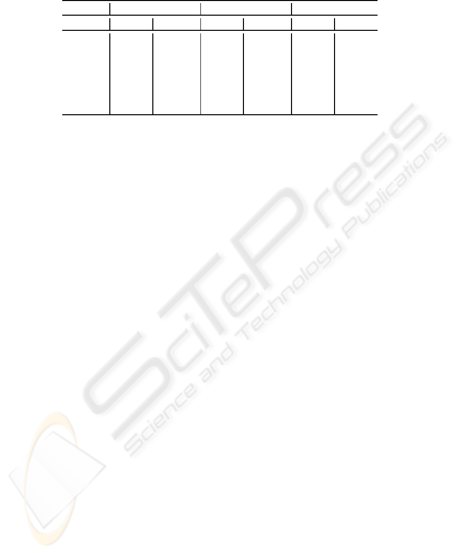
Table 4: Mean and standard deviation of sensitivity (in %) and specificity (in %) metrics on UCI data sets.
StdMLP SVM BalMLP
Data Set sens spec sens spec sens spec
Diabetes 61± 07 81± 06 70± 10 77± 04 73± 09 73 ± 04
Breast 42± 15 86± 08 60± 26 77± 08 66± 23 74 ± 11
Heart 47± 19 83± 05 61± 10 96± 09 73± 15 75± 09
Glass 84± 16 98± 02 87± 26 100± 00 90± 13 98± 03
Car 00± 00 100± 00 44 ± 21 98± 03 80± 15 77 ± 17
Yeast 06± 16 100± 00 29± 27 99± 04 82± 14 85± 03
Abalone 00 ± 00 100± 00 00± 00 100± 00 73± 12 79± 03
served that it depends on the number of class exam-
ples. We have also realized that this dependency can
be influenced by the asymptotic boundaries imposed
by the reduced size of the training and test data sets
and also by the difference in noise level between the
classes.
REFERENCES
Asuncion, A. and Newman, D. (2007). UCI machine learn-
ing repository.
Cortes, C. and Mohri, M. (2004). Auc optimization vs. error
rate minimization. In Advances in Neural Information
Processing Systems 16. MIT Press, Cambridge, MA.
Cortes, C. and Vapnik, V. (1995). Support-vector networks.
Mach. Learn., 20(3):273–297.
Egan, J. P. (1975). Signal Detection Theory and ROC Anal-
ysis. Academic Press.
Elkan, C. (2001). The foundations of cost-sensitive learn-
ing. In Proceedings of the Seventeenth International
Joint Conference on Artificial Intelligence, IJCAI,
pages 973–978.
Everson, R. M. and Fieldsend, J. E. (2006). Multi-class roc
analysis from a multi-objective optimisation perspec-
tive. Pattern Recogn. Lett., 27(8):918–927.
Fawcett, T. (2004). Roc graphs: Notes and practical consid-
erations for researchers. Technical report.
Graening, L., Jin, Y., and Sendhoff, B. (2006). General-
ization improvement in multi-objective learning. In
International Joint Conference on Neural Networks,
pages 9893–9900. IEEE Press.
Haykin, S. (1994). Neural Networks: A Comprehensive
Foundation. Macmillan, New York.
Japkowicz, N. (2000). The class imbalance problem: Sig-
nificance and strategies. In Proceedings of the 2000
International Conference on Artificial Intelligence,
pages 111–117.
Kupinski, M. A. and Anastasio, M. A. (1999). Multiobjec-
tive genetic optimization of diagnostic classifiers with
implications for generating receiver operating charac-
terisitic curves. IEEE Trans. Med. Imag., 18:675–685.
Provost, F. and Fawcett, T. (2001). Robust classification for
imprecise environments. Mach. Learn., 42(3):203–
231.
Provost, F. J., Fawcett, T., and Kohavi, R. (1998). The case
against accuracy estimation for comparing induction
algorithms. In ICML ’98: Proceedings of the Fif-
teenth International Conference on Machine Learn-
ing, pages 445–453, San Francisco, CA, USA. Mor-
gan Kaufmann Publishers Inc.
Rumelhart, D. E. and McClelland, J. L. (1986). Parallel dis-
tributed processing: Explorations in the microstruc-
ture of cognition, volume 1: Foundations. MIT Press.
Sanchez, M. S., Ortiz, M. C., Sarabia, L. A., and Lleti, R.
(2005). On pareto-optimal fronts for deciding about
sensitivity and specificity in class-modelling prob-
lems. Analytica Chimica Acta, 544(1-2):236–245.
Sun, Y., Kamel, M. S., Wong, A. K. C., and Wang, Y.
(2007). Cost-sensitive boosting for classification of
imbalanced data. Pattern Recognition, 40(12):3358–
3378.
Van Gestel, T., Suykens, J. A. K., Baesens, B., Viaene, S.,
Vanthienen, J., Dedene, G., De Moor, B., and Vande-
walle, J. (2004). Benchmarking least squares support
vector machine classifiers. Mach. Learn., 54(1):5–32.
Weiss, G. M. (2004). Mining with rarity: a unifying frame-
work. SIGKDD Explor. Newsl., 6(1):7–19.
Wu, G. and Chang, E. Y. (2005). Kba: Kernel boundary
alignment considering imbalanced data distribution.
IEEE Trans. Knowl. Data Eng., 17(6):786–795.
Zhou, Z.-H. and Liu, X.-Y. (2006). Training cost-sensitive
neural networks with methods addressing the class im-
balance problem. IEEE Trans. Knowl. Data Eng.,
18(1):63–77.
ARTIFICIAL NEURAL NETWORKS LEARNING IN ROC SPACE
489