EV
OLUTIONARY DYNAMICS OF EXTREMAL OPTIMIZATION
Stefan B
¨
ottcher
Physics Department, Emory University, Atlanta, GA 30322, U.S.A.
Keywords:
Extremal Optimization, Self-Organized Criticality, Evolution Strategies, Co-evolution and Collective Behav-
ior, Spin Glasses.
Abstract:
Motivated by noise-driven cellular automata models of self-organized criticality (SOC), a new paradigm for
the treatment of hard combinatorial optimization problems is proposed. An extremal selection process pref-
erentially advances variables in a poor local state. The ensuing dynamic process creates broad fluctuations
to explore energy landscapes widely, with frequent returns to near-optimal configurations. This Extremal
Optimization heuristic is evaluated theoretically and numerically.
1 INTRODUCTION
Physical processes have inspired many optimization
heuristics. Most famously, variants of simulated an-
nealing (Kirkpatrick et al., 1983) and genetic algo-
rithms (Goldberg, 1989) are widely used tools for the
exploration of many intractable optimization prob-
lems. But the breadth and complexity of important
real-life problems leaves plenty of room for alter-
natives to verify or improve results. One truly al-
ternative approach is the extremal optimization (EO)
method (Boettcher and Percus, 2001b). Basically, EO
focuses on eliminating only extremely bad features of
a solution while replacing them at random. Good so-
lutions emerge dynamically in an intermittent process
that explores the configuration space widely. This
method may share the evolutionary paradigm with
genetic algorithms, but assigns fitnesses to individ-
ual variables within a single configuration. Hence,
it conducts a local search of configuration space sim-
ilar to simulated annealing. But it was intentionally
conceived to leave behind the certainties (and limi-
tations) of statistical equilibrium, which depends on
a temperature schedule, instead handing control (al-
most) entirely to the update dynamics itself. In fact, as
a few simple model problems reveal, the extremal up-
date dynamics generically leads to a sharp transition
between an ergodic and a non-ergodic (“jammed”)
search regime (Boettcher and Grigni, 2002). Adjust-
ing its only free parameter to the “ergodic edge,” as
predicted by theory, indeed leads to optimal perfor-
mance in numerical experiments.
Although our understanding of EO is only at its
beginning, some quite useful applications have al-
ready been devised that have demonstrated its effi-
ciency on a variety of combinatorial (Boettcher and
Percus, 1999; Boettcher and Percus, 2001a; Boettcher
and Percus, 2004; Hoos and St
¨
utzle, 2004) and phys-
ical optimization problems (Boettcher and Percus,
2001b; Boettcher, 2003; Boettcher, 2005; Boettcher,
2009). Comparative studies with simulated anneal-
ing (Boettcher and Percus, 2000; Boettcher and Per-
cus, 1999; Boettcher, 1999) and other Metropolis
based heuristics (Dall and Sibani, 2001; Wang and
Okabe, 2003; Wang, 2003; Boettcher and Sibani,
2005; Boettcher and Frank, 2006) have established
EO as a successful alternative for the study of NP-
hard problems and its use has spread throughout the
sciences. EO has found a large number of applica-
tions by other researchers, e. g. for polymer confir-
mation studies (Shmygelska, 2007; Mang and Zeng,
2008), pattern recognition (Meshoul and Batouche,
2002b; Meshoul and Batouche, 2002a; Meshoul and
Batouche, 2003), signal filtering (Yom-Tov et al.,
2001; Svenson, 2004), transport problems (de Sousa
et al., 2004b), molecular dynamics simulations (Zhou
et al., 2005), artificial intelligence (Menai and Ba-
touche, 2002; Menai and Batouche, 2003b; Menai
and Batouche, 2003a), modeling of social networks
(Duch and Arenas, 2005; Danon et al., 2005; Neda
et al., 2006), and 3d−spin glasses (Dall and Sibani,
2001; Onody and de Castro, 2003). Also, extensions
111
Böttcher S. (2009).
EVOLUTIONARY DYNAMICS OF EXTREMAL OPTIMIZATION.
In Proceedings of the International Joint Conference on Computational Intelligence, pages 111-118
DOI: 10.5220/0002314101110118
Copyright
c
 SciTePress

(Middleton, 2004; Iwamatsu and Okabe, 2004; de
Sousa et al., 2003; de Sousa et al., 2004a) and rigor-
ous performance guarantees (Heilmann et al., 2004;
Hoffmann et al., 2004) have been established. In
(Hartmann and Rieger, 2004b) a thorough description
of EO and extensive comparisons with other heuris-
tics (such as simulated annealing, genetic algorithms,
tabu search, etc) is provided, addressed more at com-
puter scientists.
Here, we will apply EO to a spin glass model on
a 3-regular random graph to elucidate some of its dy-
namic features as an evolutionary algorithm. These
properties prove quite generic, leaving local search
with EO free of tunable parameters. We discuss
the theoretical underpinning of its behavior, which is
reminiscent of Kauffman’s suggestion (Kauffman and
Johnsen, 1991) that evolution progresses most rapidly
near the “edge of chaos,” in this case characterized by
a critical transition between a diffusive and a jammed
phase.
2 MOTIVATION: MEMORY
AND AVALANCHES IN
CO-EVOLUTION
The study of driven, dissipative dynamics has pro-
vided a plausible view of many self-organizing pro-
cesses ubiquitous in Nature (Bak, 1996). Most fa-
mously, the Abelian sandpile model (Bak et al., 1987)
has been used to describe the statistics of earth-
quakes (Bak, 1996). Another variant is the Bak-
Sneppen model (BS) (Bak and Sneppen, 1993), in
which variables are updated sequentially based on a
global threshold condition. It provides an explanation
for broadly distributed extinction events (Raup, 1986)
and the “missing link” problem (Gould and Eldredge,
1977). Complexity in these SOC models emerges
purely from the dynamics, without tuning of parame-
ters, as long as driving is slow and ensuing avalanches
are fast.
In the BS, “species” are located on the sites of
a lattice, and have an associated “fitness” value be-
tween 0 and 1. At each time step, the one species
with the smallest value (poorest degree of adaptation)
is selected for a random update, having its fitness re-
placed by a new value drawn randomly from a flat
distribution on the interval [0,1]. But the change in fit-
ness of one species impacts the fitness of interrelated
species. Therefore, all of the species at neighbor-
ing lattice sites have their fitness replaced with new
random numbers as well. After a sufficient number
of steps, the system reaches a highly correlated state
known as self-organized criticality (SOC) (Bak et al.,
1987). In that state, almost all species have reached a
fitness above a certain threshold. These species, how-
ever, possess punctuated equilibrium (Gould and El-
dredge, 1977): only ones weakened neighbor can un-
dermine ones own fitness. This co-evolutionary activ-
ity gives rise to chain reactions called “avalanches”,
large fluctuations that rearrange major parts of the
system, making any configuration accessible.
We have derived an exact delay equation
(Boettcher and Paczuski, 1996) describing the spatio-
temporal complexity of BS. The evolution of activity
P(r,t) after a perturbation at (r = 0,t = 0),
∂
t
P(r,t) = ∇
2
r
P(r,t) +
Z
t
t
0
=0
dt
0
V (t −t
0
)P(r,t
0
), (1)
with the kernel V(t) ∼ t
−γ
, has the solution P(r,t) ∼
exp{−C(r
D
/t)
1
D−1
} with D = 2/(γ −1). Thus, it is
the memory of all previous events that determines the
current activity.
Although co-evolution may not have optimization
as its exclusive goal, it serves as a powerful paradigm.
We have used it as motivation for a new approach to
approximate hard optimization problems (Boettcher
and Percus, 2000; Boettcher and Percus, 2001b; Hart-
mann and Rieger, 2004a). The heuristic we have in-
troduced, called extremal optimization (EO), follows
the spirit of the BS, updating those variables which
have among the (extreme) “worst” values in a solution
and replacing them by random values without ever
explicitly improving them. The resulting heuristic ex-
plores the configuration space Ω widely with frequent
returns to near-optimal solutions, without tuning of
parameters.
3 EXTREMAL OPTIMIZATION
FOR SPIN GLASS GROUND
STATES
Disordered spin systems on sparse random graphs
have been investigated as mean-field models of spin
glasses or combinatorial optimization problems (Per-
cus et al., 2006), since variables are long-range con-
nected yet have a small number of neighbors. Par-
ticularly simple are α-regular random graphs, where
each vertex possesses a fixed number α of bonds to
randomly selected other vertices. One can assign a
spin variable x
i
∈ {−1,+1} to each vertex, and ran-
dom couplings J
i, j
, either Gaussian or ±1, to existing
bonds between neighboring vertices i and j, leading to
competing constraints and “frustration” (Fischer and
Hertz, 1991). We want to minimize the energy of
IJCCI 2009 - International Joint Conference on Computational Intelligence
112

the system, which is the difference between violated
bonds and satisfied bonds,
H = −
∑
{bonds}
J
i, j
x
i
x
j
. (2)
EO performs a local search (Hoos and St
¨
utzle,
2004) on an existing configuration of n variables by
changing preferentially those of poor local arrange-
ment. For example, in case of the spin glass model in
Eq. (2), λ
i
= x
i
∑
j
J
i, j
x
j
assesses the local “fitness” of
variable x
i
, where H = −
∑
i
λ
i
represents the overall
energy (or cost) to be minimized. EO simply ranks
variables,
λ
Π(1)
≤ λ
Π(2)
≤ . . . ≤ λ
Π(n)
, (3)
where Π(k) = i is the index for the kth-ranked vari-
able x
i
. Basic EO always selects the (extremal) lowest
rank, k = 1, for an update. Instead, τ-EO selects the
kth-ranked variable according to a scale-free proba-
bility distribution
P(k) ∝ k
−τ
. (4)
The selected variable is updated unconditionally, and
its fitness and that of its neighboring variables are
reevaluated. This update is repeated as long as de-
sired, where the unconditional update ensures sig-
nificant fluctuations with sufficient incentive to re-
turn to near-optimal solutions due to selection against
variables with poor fitness, for the right choice of τ.
Clearly, for finite τ, EO never “freezes” into a single
configuration; it is able to return an extensive list of
the best of the configurations visited (or simply their
cost) instead (Boettcher and Percus, 2004).
For τ = 0, this “τ-EO” algorithm is simply a ran-
dom walk through configuration space. Conversely,
for τ → ∞, the process approaches a deterministic lo-
cal search, only updating the lowest-ranked variable,
and is likely to reach a dead end. However, for fi-
nite values of τ the choice of a scale-free distribution
for P(k) in Eq. (4) ensures that no rank gets excluded
from further evolution, while maintaining a clear bias
against variables with bad fitness. As Sec. 5 will
demonstrate, fixing
τ −1 ∼ 1/ ln(n) (5)
provides a simple, parameter-free strategy, activat-
ing avalanches of adaptation (Boettcher and Percus,
2000; Boettcher and Percus, 2001b).
4 EO DYNAMICS
Understanding the Dynamics of EO has proven a use-
ful endeavor (Boettcher and Grigni, 2002; Boettcher
and Frank, 2006). Such insights have lead to the im-
plementation of τ-EO described in Sec. 3. Treating τ-
EO as an evolutionary process allows us to elucidate
its capabilities and to make further refinements. Us-
ing simulations, we have analyzed the dynamic pat-
tern of the τ-EO heuristic. As described in Sec. 3,
we have implemented τ-EO for the spin glass with
Gaussian bonds on a set of instances of 3-regular
graphs of sizes n = 256, 512, and 1024, and run each
instance for T
run
= 20n
3
update steps. As a func-
tion of τ, we measured the ensemble average of the
lowest-found energy density hei = hHi/n, the first-
return time distribution R (∆t) of update activity to
any specific spin, and auto-correlations C(t) between
two configurations separated by a time t in a single
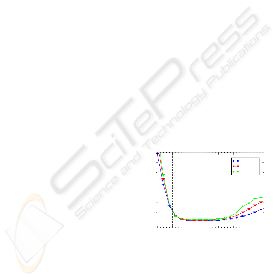
run. In Fig. 1, we show the plot of hei, which confirms
the picture found numerically (Boettcher and Percus,
2001b; Boettcher and Percus, 2001a) and theoreti-
cally (Boettcher and Grigni, 2002) for τ−EO. The
transition at τ = 1 in Eq. (5) will be investigate fur-
ther below and theoretically in Sec. 5. The worsening
behavior for large τ has been shown theoretically in
(Boettcher and Grigni, 2002) to originate with the fact
that in any finite-time application, T
run
< ∞, τ−EO be-
comes less likely to escape local minima for increas-
ing τ and n. The combination of the purely diffusive
search below τ = 1 and the “jammed” state for large
τ leads to Eq. (5), consistent with Fig. 1 and exper-
iments in (Boettcher and Percus, 2001a; Boettcher
and Percus, 2001b).
0.5
1.0
1.5
2.0
2.5
3.0
3.5
4.0
τ
-1.1
-1.0
-0.9
-0.8
<e>
n= 256
n= 512
n=1024
Figure 1: Plot of the average lowest energy density found
with τ−EO over a fixed testbed of 3-regular graph instances
of size n for varying τ. For n →∞, the results are near-
optimal only in a narrowing range of τ just above τ =1. Be-
low τ = 1 results dramatically worsen, hinting at the phase
transition in the search dynamics obtained in Sec. 5.
In Fig. 2 we show the first-return probability for
select values of τ. It shows that τ-EO is a fractal re-
newal process for all τ > 1, and for τ < 1 it is a Pois-
son process: when variables are drawn according to
EVOLUTIONARY DYNAMICS OF EXTREMAL OPTIMIZATION
113

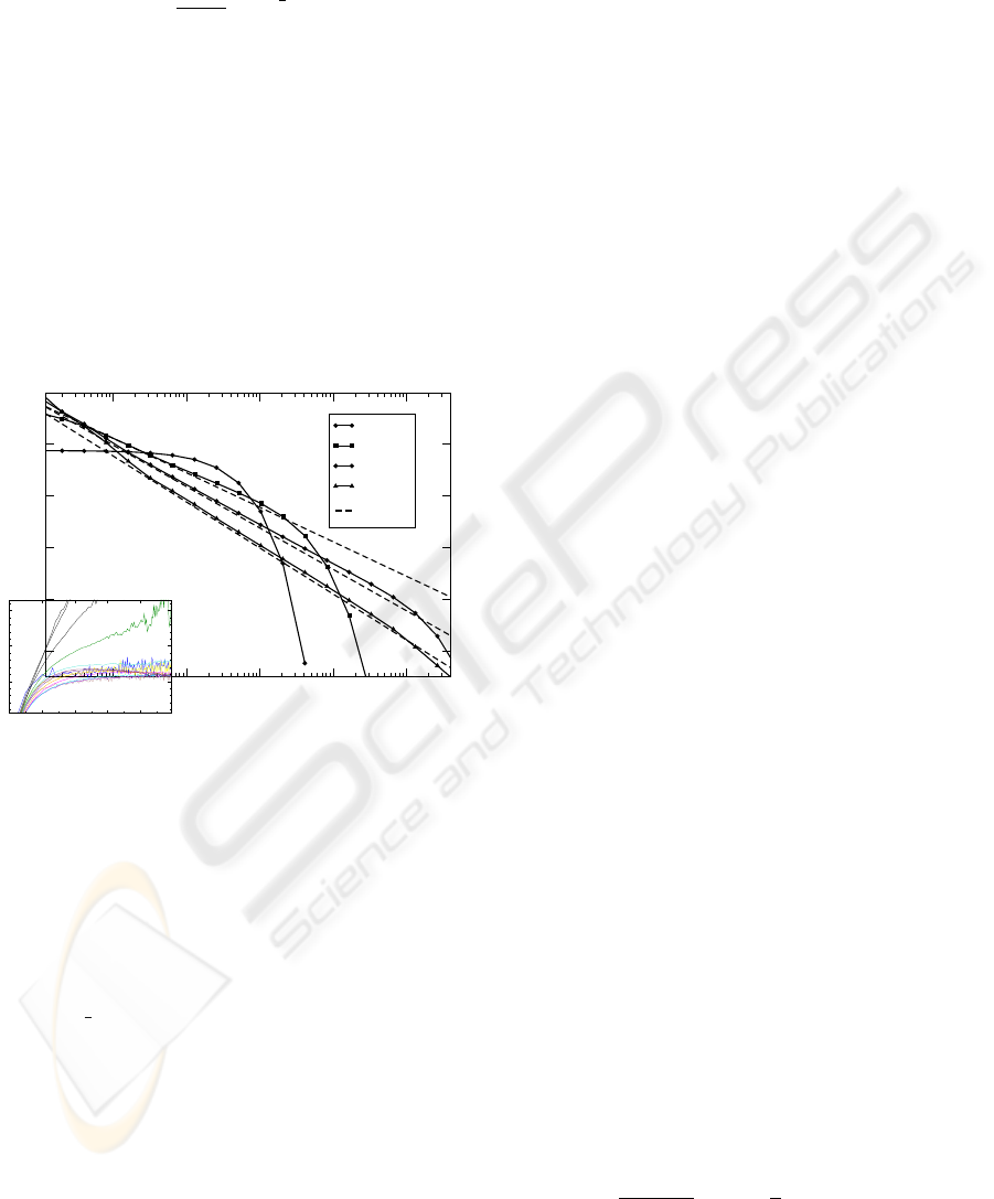
their “rank” k with probability P(k) in Eq. (3), one
gets for the first-return time distribution
R(∆t) ∼−
P(k)
3
P
0
(k)
∼ ∆t
1
τ
−2
. (6)
Neglecting correlations between variables, the num-
ber of updates of a variable of rank k is #(k) =
T
run
P(k). Then, the typical life-time is ∆t(k) ∼
T
run
/#(k) = 1/P(k), which via R(∆t)d∆t = P(k)dk
immediately gives Eq. (6). The numerical results in
Fig. 2 fit the prediction in Eq. (6) well. Note that the
average life-time, and hence the memory preserved
by each variable, diverges for all τ(> 1), limited only
by T
run
, a size-dependent cut-off, and is widest for
τ → 1
+
, where τ-EO performs optimal. This finding
affirms the subtle relation between searching config-
uration space widely while preserving the memory of
good solutions.
10
1
10
2
10
3
10
4
10
5
∆t
10
-10
10
-8
10
-6
10
-4
10
-2
R(∆t)
τ=0.2
τ=1.5
τ=2.5
τ=4.5
∆t
1/τ-2
0 20 40 60 80
t
1/2
3
4
5
[d(ln C)/d(t
1/2
)]/B
τ
Figure 2: Plot of the first-return time distribution R(∆t)
for τ-EO for various τ and n = 256. Poissonian behav-
ior for τ < 1 develops into a power-law regime limited by
a cut-off for τ > 1. The power-law scaling closely fol-
lows Eq. (6) (dashed lines). Inset: Data collapse (ex-
cept for τ ≤ 1) of autocorrelations C(t) according to the
stretched-exponential fit given in the text. From top to bot-
tom, τ = 0.5,0.7,... ,3.5.
Interestingly, the auto-correlations between con-
figurations shown in the inset of Fig. 2 appear
to decay with a stretched-exponential tail, C(t) ∼
exp{−B
τ
√
t} fitted with B
τ
≈ 1.6 exp{−2.4τ}, for all
τ > 1, characteristic of a super-cooled liquid (Fis-
cher and Hertz, 1991) just above the glass transition
temperature T
g
(> 0 in this model). While we have
not been able to derive that result, it suggests that τ-
EO, driven far from equilibrium, never “freezes” into
a glassy (T < T
g
) state, yet accesses T = 0 proper-
ties efficiently. Such correlations typically decay with
an agonizingly anemic power-law (Fischer and Hertz,
1991) for local search of a complex energy landscape,
entailing poor exploration and slow convergence.
5 THEORETICAL
INVESTIGATIONS
Despite the general difficulty in predicting perfor-
mance features for stochastic heuristics (Lundy and
Mees, 1996; Aarts and van Laarhoven, 1987), we are
able to theoretically extract a few non-trivial prop-
erties of τ-EO. We have studied a general model
problem for which the asymptotic behavior of τ-EO
can be solved exactly (Boettcher and Grigni, 2002;
Boettcher and Frank, 2006). The model obtains
Eq. (5) exactly in cases where the model develops a
“jam” amongst its variables, a generic feature of frus-
trated systems.
To analyze the properties of the τ-EO update pro-
cess, we have to access the fitness of individual vari-
ables. Our model (Boettcher and Grigni, 2002) con-
sists of n a priori independent (“annealed”) variables
x
i
, taking on one of, say, three fitness states, λ
i
= 0,
−1, or −2. At each point in time, respective fractions
ρ
0
, ρ
1
, and ρ
2
of the variables occupy these states,
where
∑
a
ρ
a
= 1. The optimal configuration is ρ
0
= 1,
ρ
1,2
= 0 with a cost per variable of C = −
∑
i
λ
i
/n =
∑
2
a=0
aρ
a
= 0, according to Eq. (3). With this sys-
tem, we can model the dynamics of a local search
for hard problems by “designing” an interesting set
of flow equations for ρ(t) that can mimic a complex
search space Ω with energetic and entropic barriers.
In these flow equations, a transition matrix T
ab
speci-
fies what fraction of variables transitions in or out of a
fitness state (a), given that a variable in a certain state
(b) is updated. (This transition of a is conditioned by
b, not necessarily between a and b!) The probabilities
for the condition that a variable in ρ
b
is updated, Q
b
,
can be derived exactly for local search,
˙
ρ
a
=
∑
b
T
ab
Q
b
, (7)
typically giving a highly non-linear dynamic system.
For example, for τ-EO the vector Q depends exclu-
sively on ρ, since for each update a variable is selected
based only on its rank according to Eq. (5). When
a rank k(≤ n) has been chosen, a spin is randomly
picked from state 0 ≤ a ≤ α(= 2 here), if k/n ≤ ρ
α
,
from state α −1, if ρ
α
< k/n ≤ ρ
α
+ ρ
α−1
, and so
on. We introduce a new, continuous variable x = k/n
(n À 1), and rewrite P(k) in Eq. (5) as
p(x) =
τ −1
n
τ−1
−1
x
−τ
µ
1
n
≤ x ≤ 1
¶
, (8)
where the maintenance of the low-x cut-off at 1/n will
turn out to be crucial. Now, the average likelihood
IJCCI 2009 - International Joint Conference on Computational Intelligence
114

that a spin in a given state is updated is given by
Q
α
=
Z
ρ
α
1/n
p(x)dx =
ρ
1−τ
α
−n
τ−1
1 −n
τ−1
,
Q
α−1
=
Z
ρ
α
+ρ
α−1
ρ
α
p(x)dx
=
(ρ
α−1
+ ρ
α
)
1−τ
−ρ
1−τ
α
1 −n
τ−1
, (9)
...
Q
0
=
Z
1
1−ρ
0
p(x)dx =
1 −(1 −ρ
0
)
1−τ
1 −n
τ−1
,
where in the last line the norm
∑
i
ρ
i
= 1 was used in
both integration limits. These values of the Q’s com-
pletely describe the update preferences for τ-EO at
arbitrary τ. In the case α = 2, Eq. (10) gives
Q
0
=
1 −(1 −ρ
0
)
1−τ
1 −n
τ−1
, Q
1
=
(ρ
1
+ ρ
2
)
1−τ
−ρ
1−τ
2
1 −n
τ−1
,
and Q
2
= 1 − Q
0
− Q
1
. We can compare with
any other local search heuristics, such as sim-
ulated annealing (SA) (Kirkpatrick et al., 1983)
with temperature schedule β = 1/T = β(t), where
Metropolis-updates require (Boettcher and Grigni,
2002; Boettcher and Frank, 2006)
Q
a
∝ ρ
a
min
(
1,exp
"
−β
α
∑
b=0
bT
ba
#)
, (10)
for a = 0,1,..,α. Thus, with the choice of a specific
model T, we could study any (dynamic or stationary)
property of τ-EO as a function of τ and compare it to
SA.
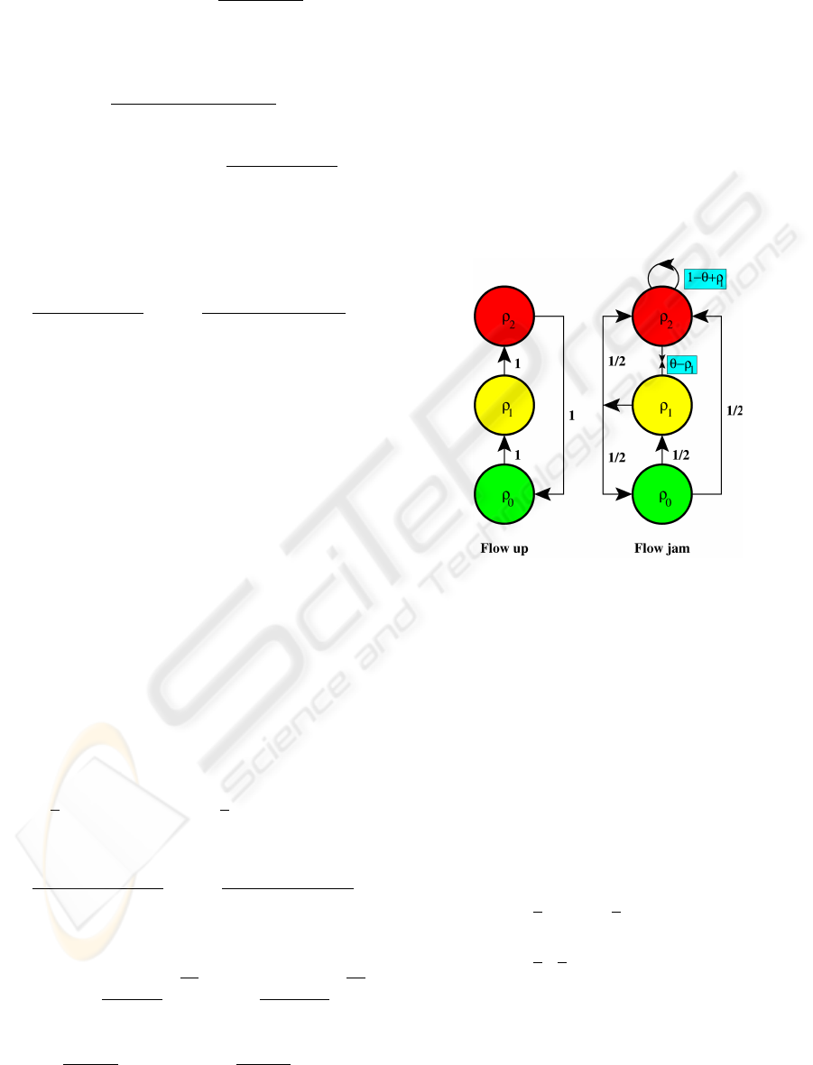
To demonstrate the use of these equations, we
consider a (trivial) model with a constant matrix
describing the transition of fractions of variables,
T
ab
= [−δ
ab
+ δ
(2+a mod 3),b
]/n, depicted on the left
in Fig. 3. Here, variables in ρ
1
can only reach the
lowest-energy state in ρ
0
by first jumping up in energy
to ρ
2
. Using
˙
ρ
2
= −
˙
ρ
0
−
˙
ρ
1
, since ρ
0
+ ρ
1
+ ρ
2
= 1,
Eq. (7) gives
˙
ρ
0
=
1
n
(−Q
0
+ Q
2
),
˙
ρ
1
=
1
n
(Q
0
−Q
1
), (11)
with Q in Eq. (10) for EO and for SA with
Q
0
=
ρ
0
e
−β
(1 −e
−β
)ρ
2
+ e
−β
, Q
1
=
ρ
1
e
−β
(1 −e
−β
)ρ
2
+ e
−β
.
The stationary solution, for
˙
ρ = 0, yields Q
0
= Q
1
=
Q
2
, and gives for EO and SA:
EO : ρ
0
=1−
µ
n
τ−1
+ 2
3
¶
1
1−τ
,ρ
2
=
µ
2n
τ−1
+ 1
3
¶
1
1−τ
SA : ρ
0
=
1
2 + e
−β
, ρ
2
=
e
−β
2 + e
−β
. (12)
and ρ
1
= 1 −ρ
0
−ρ
2
. Therefore, SA reaches its best,
albeit suboptimal, cost C = 1/2 > 0 at β → ∞, due
to the energetic barrier faced by the variables in ρ
1
.
The result for EO is most remarkable (Boettcher and
Grigni, 2002; Boettcher and Frank, 2006): For n → ∞
at τ < 1 EO remains suboptimal, but reaches the op-
timal cost for all τ > 1! This transition at τ = 1 sepa-
rates an (ergodic) random walk phase with too much
fluctuation, and a greedy-descent phase with too lit-
tle fluctuation, which in real NP-hard problems would
probably produce broken ergodicity (Bantilan and
Palmer, 1981). This “ergodicity breaking” derives
from the scale-free power-law in Eq. (5) (Boettcher
and Percus, 2000).
Figure 3: Plot of flow diagrams. In the diagram on the left,
variables have to jump to higher energetic states first before
they can attain the lowest state. The right diagram shows
the model of a jam, where variables in the highest state can
only traverse through the intermediate state to the lowest
state, if the intermediate state moves its variables out of the
way first to keep its density ρ
1
below the threshold θ.
Naturally, the range of phenomena found in a lo-
cal search of NP-hard problems is not limited to en-
ergetic barriers. After all, so far we have only con-
sidered constant entries for T
i, j
. In our next model we
let T merely depend linearly on the ρ
i
. Most of these
cases reduce to the phenomena already discussed in
the previous example. An entirely new effect arises in
the case depicted on the right in Figure 3:
˙
ρ
0
=
1
n
·
−Q
0
+
1
2
Q
1
¸
, (13)
˙
ρ
1
=
1
n
·
1
2
Q
0
−Q
1
+ (θ −ρ
1
)Q
2
¸
.
Aside from the dependence of T on ρ
1
, we have also
introduced the threshold parameter θ. The interesting
regime is the case 0 < θ < 1, where further flow from
state 2 into state 1 can be blocked for increasing ρ
1
,
EVOLUTIONARY DYNAMICS OF EXTREMAL OPTIMIZATION
115

providing a negative feedback to the system. In ef-
fect, the model may exhibit a “jam” typical in glassy
dynamics and in local search heuristics.
Eqs. (14) again have a unique fixed-point solution
with τ = ∞ being the most favorable value at which
the minimal energy C = 0 is definitely reached. But
it can be shown that the system has an ever harder
time to reach that point, requiring typically t = O(n
τ
)
update steps for a finite fraction of initial condi-
tions. Thus, for a given finite computational time
t
max
the best results are obtained at some finite value
of τ
opt
. In that, this model provides a new feature –
slow variables impeding the dynamics of faster ones
(Palmer et al., 1984) – resembling the observed be-
havior for EO on real problems, e.g. the effect shown
in Fig. 1. In particular, this model provides an ana-
lytically tractable picture for the relation between the
value of τ
opt
and the effective loss of ergodicity in the
search conjectured in (Boettcher and Percus, 2000;
Boettcher and Percus, 2001a).
For initial conditions that lead to a jam, ρ
1
(0) +
ρ
2
(0) > θ, we assume that
ρ
1
(t) = θ −ε(t) (14)
with ε ¿ 1 for t ≤t
jam
, where t
jam
is the time at which
ρ
2
becomes small and Eq. (14) fails. To determine
t
jam
, we apply Eq. (14) to the evolution equations in
(14) and obtain after some calculation (Boettcher and
Grigni, 2002)
t
jam
∼ n
τ
, (15)
Further analysis shows that the average cost hCi
τ
develops a minimum when t
max
∼t
jam
for t
max
> n, so
choosing t
max
= an leads directly to Eq. (5) for τ
opt
.
This sequence of minima in hCi(τ) for increasing n
is confirmed by the numerical simulations (with a =
100) shown in Fig. 1, with the correct n-dependence
predicted by Eq. (5).
6 NUMERICAL RESULTS FOR
EO
To gauge τ-EO’s performance for larger 3d-lattices,
we have run our implementation also on two in-
stances, toruspm3-8-50 and toruspm3-15-50, with
n = 512 and n = 3375, considered in the 7th DIMACS
challenge for semi-definite problems
1
. The best avail-
able bounds (thanks to F. Liers) established for the
larger instance are H
lower
= −6138.02 (from semi-
definite programming) and H
upper
= −5831 (from
branch-and-cut). EO found H
EO
= −6049 (or H/n =
1
http://dimacs.rutgers.edu/Challenges/Seventh/
−1.7923), a significant improvement on the up-
per bound and already lower than lim
n→∞
H/n ≈
−1.786... found in (Boettcher and Percus, 2001b).
Furthermore, we collected 10
5
such states, which
roughly segregate into three clusters with a mutual
Hamming distance of at least 100 distinct spins;
though at best a small sample of the ≈ 10
73
ground
states expected (Hartmann, 2001)! For the smaller in-
stance the bounds given are −922 and −912, while
EO finds −916 (or H/n = −1.7891) and was termi-
nated after finding 10
5
such states.
7 CONCLUSIONS
We have motivated the Extremal Optimization heuris-
tic and reviewed briefly some of its previous applica-
tions. Using the example of Ising spin glasses, which
is equivalent to combinatorial problems with con-
straint Boolean variables such as satisfiability or col-
oring, we have thoroughly described its implementa-
tion and analyzed its evolution, numerically and theo-
retically. The new paradigm of using the dynamics of
extremal selection, i. e. merely eliminating the worst
instead of freezing in the perceived good, is shown
to yield a highly flexible and adaptive search routine
that explores widely and builds up memory systemat-
ically. It is the dynamics more than any fine-tuning of
parameters that determines its success. These results
are largely independent of the specific implementa-
tion used here and beg for applications to other com-
binatorial problems in science and engineering.
ACKNOWLEDGEMENTS
I would like to thank M. Paczuski, A.G. Percus, and
M. Grigni for their collaboration on many aspects of
the work presented here. This work was supported
under NSF grants DMR-0312510 and DMR-0812204
and the Emory University Research Committee.
REFERENCES
Aarts, E. H. L. and van Laarhoven, P. J. M. (1987). Sim-
ulated Annealing: Theory and Applications. Reidel,
Dordrecht.
Bak, P. (1996). How Nature works: The Science of Self-
Organized Criticality. Copernicus, New York.
Bak, P. and Sneppen, K. (1993). Punctuated equilibrium
and criticality in a simple model of evolution. Phys.
Rev. Lett., 71:4083–4086.
IJCCI 2009 - International Joint Conference on Computational Intelligence
116

Bak, P., Tang, C., and Wiesenfeld, K. (1987). Self-
organized criticality: An explanation of the 1/f noise.
Phys. Rev. Lett., 59(4):381–384.
Bantilan, F. T. and Palmer, R. G. (1981). Magnetic prop-
erties of a model spin glass and the failure of linear
response theory. J. Phys. F: Metal Phys., 11:261–266.
Boettcher, S. (1999). Extremal optimization and graph par-
titioning at the percolation threshold. J. Math. Phys.
A: Math. Gen., 32:5201–5211.
Boettcher, S. (2003). Numerical results for ground states
of mean-field spin glasses at low connectivities. Phys.
Rev. B, 67:R060403.
Boettcher, S. (2005). Extremal optimization for
Sherrington-Kirkpatrick spin glasses. Eur. Phys. J. B,
46:501–505.
Boettcher, S. (2009). Simulations of Energy Fluctuations in
the Sherrington-Kirkpatrick Spin Glass. (submitted)
arXiv:0906.1292.
Boettcher, S. and Frank, M. (2006). Optimizing at the er-
godic edge. Physica A, 367:220–230.
Boettcher, S. and Grigni, M. (2002). Jamming model for
the extremal optimization heuristic. J. Phys. A: Math.
Gen., 35:1109–1123.
Boettcher, S. and Paczuski, M. (1996). Ultrametricity and
memory in a solvable model of self-organized critical-
ity. Phys. Rev. E, 54:1082.
Boettcher, S. and Percus, A. G. (1999). Extremal opti-
mization: Methods derived from co-evolution. In
GECCO-99: Proceedings of the Genetic and Evo-
lutionary Computation Conference, pages 825–832,
Morgan Kaufmann, San Francisco.
Boettcher, S. and Percus, A. G. (2000). Nature’s way of
optimizing. Artificial Intelligence, 119:275.
Boettcher, S. and Percus, A. G. (2001a). Extremal optimiza-
tion for graph partitioning. Phys. Rev. E, 64:026114.
Boettcher, S. and Percus, A. G. (2001b). Optimization with
extremal dynamics. Phys. Rev. Lett., 86:5211–5214.
Boettcher, S. and Percus, A. G. (2004). Extremal optimiza-
tion at the phase transition of the 3-coloring problem.
Phys. Rev. E, 69:066703.
Boettcher, S. and Sibani, P. (2005). Comparing extremal
and thermal explorations of energy landscapes. Eur.
Phys. J. B, 44:317–326.
Dall, J. and Sibani, P. (2001). Faster Monte Carlo
Simulations at Low Temperatures: The Waiting
Time Method. Computer Physics Communication,
141:260–267.
Danon, L., Diaz-Guilera, A., Duch, J., and Arenas, A.
(2005). Comparing community structure identifica-
tion. J. Stat. Mech.-Theo. Exp., P09008.
de Sousa, F. L., Ramos, F. M., Galski, R. L., and Muraoka,
I. (2004a). Generalized extremal optimization: A new
meta-heuristic inspired by a model of natural evolu-
tion. Recent Developments in Biologically Inspired
Computing.
de Sousa, F. L., Vlassov, V., and Ramos, F. M. (2003). Gen-
eralized Extremal Optimization for solving complex
optimal design problems. Lecture Notes in Computer
Science, 2723:375–376.
de Sousa, F. L., Vlassov, V., and Ramos, F. M. (2004b).
Heat pipe design through generalized extremal opti-
mization. Heat Transf. Eng., 25:34–45.
Duch, J. and Arenas, A. (2005). Community detection
in complex networks using Extremal Optimization.
Phys. Rev. E, 72:027104.
Fischer, K. H. and Hertz, J. A. (1991). Spin Glasses. Cam-
bridge University Press, Cambridge.
Goldberg, D. E. (1989). Genetic Algorithms in Search, Op-
timization, and Machine Learning. Addison-Wesley,
Reading.
Gould, S. and Eldredge, N. (1977). Punctuated equilibria:
The tempo and mode of evolution reconsidered. Pale-
obiology, 3:115–151.
Hartmann, A. K. and Rieger, H., editors (2004a). New Op-
timization Algorithms in Physics. Springer, Berlin.
Hartmann, A. K. (2001). Ground-state clusters of two-
, three-, and four-dimensional ±J Ising spin glasses.
Phys. Rev. E, 63.
Hartmann, A. K. and Rieger, H. (2004b). New Optimization
Algorithms in Physics. Wiley-VCH, Berlin.
Heilmann, F., Hoffmann, K. H., and Salamon, P. (2004).
Best possible probability distribution over Extremal
Optimization ranks. Europhys. Lett., 66:305–310.
Hoffmann, K. H., Heilmann, F., and Salamon, P. (2004).
Fitness threshold accepting over Extremal Optimiza-
tion ranks. Phys. Rev. E, 70:046704.
Hoos, H. H. and St
¨
utzle, T. (2004). Stochastic Local Search:
Foundations and Applications. Morgan Kaufmann,
San Francisco.
Iwamatsu, M. and Okabe, Y. (2004). Basin hopping with
occasional jumping. Chem. Phys. Lett., 399:396–400.
Kauffman, S. A. and Johnsen, S. (1991). Coevolution to
the edge of chaos: Coupled fitness landscapes, poised
states, and coevolutionary avalanches. J. Theor. Biol.,
149:467–505.
Kirkpatrick, S., Gelatt, C. D., and Vecchi, M. P. (1983). Op-
timization by simulated annealing. Science, 220:671–
680.
Lundy, M. and Mees, A. (1996). Convergence of an Anneal-
ing Algorithm. Math. Programming, 34:111–124.
Mang, N. G. and Zeng, C. (2008). Reference energy ex-
tremal optimization: A stochastic search algorithm
applied to computational protein design. J. Comp.
Chem., 29:1762–1771.
Menai, M. E. and Batouche, M. (2002). Extremal Opti-
mization for Max-SAT. In Proceedings of the Inter-
national Conference on Artificial Intelligence (IC-AI),
pages 954–958.
Menai, M. E. and Batouche, M. (2003a). A Bose-Einstein
Extremal Optimization method for solving real-world
instances of maximum satisfiablility. In Proceedings
of the International Conference on Artificial Intelli-
gence (IC-AI), pages 257–262.
EVOLUTIONARY DYNAMICS OF EXTREMAL OPTIMIZATION
117

Menai, M. E. and Batouche, M. (2003b). Efficient ini-
tial solution to Extremal Optimization algorithm for
weighted MAXSAT problem. Lecture Notes in Com-
puter Science, 2718:592–603.
Meshoul, S. and Batouche, M. (2002a). Ant colony system
with extremal dynamics for point matching and pose
estimation. In 16th International Conference on Pat-
tern Recognition (ICPR’02), volume 3, page 30823.
Meshoul, S. and Batouche, M. (2002b). Robust point cor-
respondence for image registration using optimization
with extremal dynamics. Lecture Notes in Computer
Science, 2449:330–337.
Meshoul, S. and Batouche, M. (2003). Combining Extremal
Optimization with singular value decomposition for
effective point matching. Int. J. Pattern Rec. and AI,
17:1111–1126.
Middleton, A. A. (2004). Improved Extremal Optimization
for the Ising spin glass. Phys. Rev. E, 69:055701(R).
Neda, Z., Florian, R., Ravasz, M., Libal, A., and Gy
¨
orgyi,
G. (2006). Phase transition in an optimal clusteriza-
tion model. Physica A., 362:357–368.
Onody, R. N. and de Castro, P. A. (2003). Optimization and
self-organized criticality in a magnetic system. Phys-
ica A, 322:247–255.
Palmer, R. G., Stein, D. L., Abraham, E., and Anderson,
P. W. (1984). Models of hierarchically constrained dy-
namics for glassy relaxation. Phys. Rev. Lett., 53:958–
961.
Percus, A., Istrate, G., and Moore, C. (2006). Compu-
tational Complexity and Statistical Physics. Oxford
University Press, New York.
Raup, M. (1986). Biological extinction in earth history. Sci-
ence, 231:1528–1533.
Shmygelska, A. (2007). An extremal optimization search
method for the protein folding problem: the go-model
example. In GECCO ’07: Proceedings of the 2007
GECCO conference companion on Genetic and evo-
lutionary computation, pages 2572–2579, New York,
NY, USA. ACM.
Svenson, P. (2004). Extremal Optimization for sensor report
pre-processing. Proc. SPIE, 5429:162–171.
Wang, J. (2003). Transition matrix Monte Carlo and flat-
histogram algorithm. In AIP Conf. Proc. 690: The
Monte Carlo Method in the Physical Sciences, pages
344–348.
Wang, J.-S. and Okabe, Y. (2003). Comparison of Extremal
Optimization with flat-histogram dynamics for finding
spin-glass ground states. J. Phys. Soc. Jpn., 72:1380.
Yom-Tov, E., Grossman, A., and Inbar, G. F. (2001).
Movement-related potentials during the performance
of a motor task i: The effect of learning and force.
Biological Cybernatics, 85:395–399.
Zhou, T., Bai, W.-J., Cheng, L.-J., and Wang, B.-H. (2005).
Continuous Extremal Optimization for Lennard-Jones
clusters. Phys. Rev. E, 72:016702.
IJCCI 2009 - International Joint Conference on Computational Intelligence
118