RANDOM VARIATES GENERATING METHODS OF

TIME-BETWEEN-FAILURES FOR THE REPAIRABLE

SYSTEMS UNDER AGE-REDUCTION

PREVENTIVE MAINTENANCE

Chun-Yuan Cheng

Dept. of Industrial Engineering and Management, Chaoyang University of Technology

168, Jifong E. Rd., Wufong, Taichung County, 41349, Taiwan

Renkuan Guo

Department of Statistical Sciences, University of Cape Town, Cape Town, South Africa

Mei-Ling Liu

Dept. of Industrial Engineering and Management, National Taipei University of Technology, Taipei, Taiwan

The Office of Academic Affairs, Chaoyang University of Technology, Taichung County, Taiwan

Keywords: Simulation method, Time-between-failure random variates, Preventive maintenance, Age reduction.

Abstract: Based on the theoretical model, a numerical method is usually necessary for obtaining the optimal

preventive maintenance (PM) policy for a deteriorating system since the theoretical model becomes

complicated when the system’s hazard rate function is changed after each PM. It makes the application of

the theoretical model not suitable for real cases. Moreover, the theoretical model assumes using infinite

time span to obtain the long-term expected number of failures. Yet, in reality, the deteriorating systems

always have a finite life time. Hence, an optimal solution might not be resulted as compared to the infinite

time span. Therefore, we consider using the simulation method to obtain a range of the near-optimal PM

policy. The critical step of the simulation method for obtaining a near-optimal PM policy is the generation

of the random variates (RV). In this research, three methods are developed to generate the required RVs of

the time-between-failures (TBF) for the finite-time-span preventive maintenance model with age reduction

effect. It is found that there are no significant differences among three proposed RV generating methods

when comparing the dispersion of the generated RV’s. However, the rejection method is the simplest

method for obtaining the near-optimal PM policies. Examples of the near-optimal PM policies are also

presented in this paper.

1 INTRODUCTION

Based on the theoretical model, a numerical method

is usually necessary for finding the optimal

preventive maintenance (PM) policy for a

deteriorating system since the theoretical model

becomes complicated when the system’s hazard rate

function is changed after each PM. It makes the

application of the theoretical model not suitable for

real cases. Furthermore, by the theoretical model,

the optimal policy is obtained based on the long-

term failures occurrence under the assumption of the

infinite time span. Yet, in reality, the life time of a

system is always finite. Hence, the optimal solution

from the theoretical model may not suitable for a

single system with finite life time. In practical, a

near-optimal PM policy might be good enough for

the real applications. In order to obtain a near-

optimal PM policy for the real situations, the

simulation method is applied to generate random

variates (RV) of the time between failures (TBF).

However, recent literature survey has shown that

325

Cheng C., Guo R. and Liu M. (2009).

RANDOM VARIATES GENERATING METHODS OF TIME-BETWEEN-FAILURES FOR THE REPAIRABLE SYSTEMS UNDER AGE-REDUCTION

PREVENTIVE MAINTENANCE.

In Proceedings of the 6th International Conference on Informatics in Control, Automation and Robotics - Robotics and Automation, pages 325-330

DOI: 10.5220/0002219903250330

 SciTePress

little research has been done to obtain a near-optimal

PM policy by using the simulation method.

The critical step of the simulation method for

obtaining a near-optimal PM policy is the generation

of the random variates (RV). In this research, three

methods are developed to generate the required RVs

of the time-between-failures (TBF) for the finite-

time-span PM model with age reduction effect.

Based on the simulation method developed by

Cheng (2005), the first proposed method applies the

inverse transformation method to generate the

random variates (RV) of the time between failures

(TBF) for a PM model with age reduction effect.

The algorithm assumes that the occurrence time of

the last failure in the i

PM cycle is irrelative to the

occurrence time of the first failure in the i+1

cycle. This RV generating method for the TBF is

called “the offset inverse transformation method” in

this paper.

Intuitively, however, the occurrence time of the

first failure in the i+1

PM cycle is affected by the

occurrence time of the last failure in the i

PM cycle

since the failure occurrence of the system follows

the non-homogenous Poisson process (NHPP) and

the PM is imperfect (i.e., the PM will not renew the

system to zero failure rate). Therefore, in this

research, we have developed a modified inverse

transformation method for generating the RVs of the

TBF which is called “the trace-back inverse

transformation method”. The second proposed

method assumes the occurrence time of the first

failure in the i+1

PM cycle is affected by the

occurrence time of the last failure in the i

cycle.

Furthermore, since the rejection method is often

applied to generating RVs of complicated

distributions, we also present the third proposed

method, the rejection method, for generating the

RVs of the TBF under the age-reduced PM model.

In this paper, the algorithms and the simulation

results for the above three RV generating methods

are presented and compared. An example of finding

the near-optimal PM policy is provided by using the

rejection method of RV generation.

2 THE BACKGROUND FOR THE

THEORITICAL MODEL

2.1 Nomenclature

L the finite life time span for the system or

equipment

T the time interval of each periodic PM

N the number of PM performed in the finite

life time span (L)

the generated number of failures in the i

cycle, i = 0, 1, …, N

i,j

the generated time between the j-1

and the

failures in the i

PM cycle, i = 0, 1, …, N;

j = 1, 2, …, k

i,j

the generated occurrence time of the j

failure in the i

PM cycle where t

i,j

= t

i,j-1

1, +

the generated time between the last (k

) and

the k

failures (not existing) in the i

cycle

1, +

the generated occurrence time of k

failure (not existing) in the i

PM cycle, i.e.,

1, +

exceed the time of the i

PM cycle

γ the reduced age after each PM

i,j

the generated effective occurrence time (age)

of the j

failure in the i

PM cycle where w

i,j

= t

-iγ

i,j

the random number required for the

generation of x

λ(t) Original hazard rate function (before the 1

PM action)

(t) Hazard rate function at time t where t is in

the i

PM cycle and λ

(t)=λ(t)

F(t) the cumulated distribution function (CDF) of

the TBF at age t

R(t) the reliability at age t

Cost of each PM

Minimal repair cost of each failure

TC The total maintenance cost function in the

finite life time span

2.2 Assumptions

y The system has a finite useful life time L.

The system is deteriorating and repairable over

time where the failure process follows the non-

homogenous Poisson Process (NHPP) with

increasing failure rate (IFR). Weibull distribution

with hazard rate function:

)(

−

⎟

⎠

⎞

⎜

⎝

⎛

⎟

⎠

⎞

⎜

⎝

⎛

θθ

is used to

illustrate the examples in this paper, where

the shape parameter and

is the scale parameter.

y The periodic PM actions with constant interval (T)

are performed over the finite time span L.

y The system’s age can be reduced γ units of time to

result in a younger age (called the effective age)

after each PM. Hence, the hazard rate function at

time t

i,j

in the i

PM cycle can be written as

ICINCO 2009 - 6th International Conference on Informatics in Control, Automation and Robotics

326

i,j

) =

i,j

-iγ) =

i,j

(1)

y Minimal repair is performed when failure occurs

between each PM.

y The time required for performing PM, minimal

repair, or replacement is negligible.

2.3 The Theoretical Model

Based on the theoretical PM model with age

reduction proposed by Cheng et al. (2004) and Yeh

and Chen (2006), the optimal PM policy is obtained

by the following steps. The first step is to find the

expected cost rate function for the PM model as

shown below.

(1) (,)

(, ) ,

pm pr mr

NC CCTN

CT N

−++Λ

(2)

where Λ(T, N) is the expected number of failures

occurred in the finite time span and is defined as

(1)

(, ) ()

TN tdt

−

Λ=

∑

∫

(3)

with λ

(·) being defined in Eq. (1). Second step is to

obtain the time interval of PM (T) as a function of N

by taking the partial derivative of T of the above

expected cost rate function and letting it equal to

zero, i.e.,

(, )

CT N

∂

Third, the optimal value T

and N

of the

theoretical model can be obtained by numerically

searching

min ( , ),

CT N

N = 1, 2, … since the cost

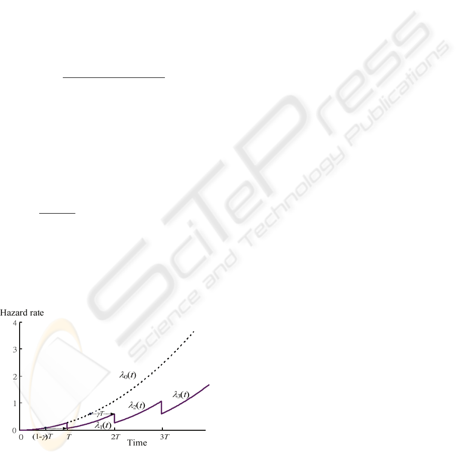
rate function is a convex function. The hazard rate

function of the PM model with age reduction is

illustrated in Figure 1.

Figure 1: The hazard rate function of the PM Model with

age reduction.

3 THE RV GENERATING

METHODS OF THE TBF

3.1 The Offset Inverse Transformation

Method

This RV generating method assumes that the

occurrence time of the last failure in the i

PM cycle

is irrelative to the occurrence time of the first failure

in the i+1

PM cycle. Thus, when the generated

occurrence time of the k

failure is within the i

cycle but the occurrence time of the k

failure

exceeds the i

PM cycle, i.e.,

> iT, we discard

the k

failure and start to generate the occurrence

time for the first failure of the i+1

PM cycle.

According to the concept of the inverse

transformation method, if x is the time between

failures, then, we have

U = F(x). (4)

However, since the PM model assumes that the

minimal repair is performed at each failure occurred

between each PM. Therefore, we can re-write Eq.(4)

i,j

= F(x

i,j

i,j-1

) = 1 - R(x

i,j

i,j-1

). (5)

Then, for the age-reduction PM model, we apply

Eq.(1) to Eq. (5) and it can be resulted as the

following equation.

{

}

,1 ,

,,,-1

1(|)exp (')'

for 0,1,..., ; 1, 2,...,

ij ij

ij ij ij i

URxt tdt

iNj k

−

−= = −

∫

(6)

which, according to Eq. (1), can be expressed as

function of effective age as follows.

{

}

,1 ,

,,,-1

1(|)exp ()

for 0,1,..., ; 1, 2,..., .

ij ij

ij ij ij

URxt tdt

iNjk

−

−= = −

∫

(7)

where w

0,j

= t

0,j

, w

i,0

= t

i,0

– iγ = iT - iγ; w

i,j

= t

i,j

– iγ =

i,j-1

+ x

i,j

– iγ. When the TBF of a system is a

Weibull random variable, based in Eq. (7), we can

generate the TBF random variates by the following

equation.

{

}

,,1,1

ln(1 )

for 0,1,..., ; 1, 2,..., .

ij ij ij ij

Uti ti

iNjk

γγ

−−

⎡⎤

−−+− −+

⎣⎦

(8)

The algorithm for the offset inverse

transformation method is presented as follows.

(1) Specify the values of the following parameters:

, N, T, L and let i = 0.

RANDOM VARIATES GENERATING METHODS OF TIME-BETWEEN-FAILURES FOR THE REPAIRABLE

SYSTEMS UNDER AGE-REDUCTION PREVENTIVE MAINTENANCE

327

(2) Let t

i,0

= iT.

(3) Let j = 1.

(4) Generate random number U

i,j

(5) Obtain the value of x

i,j

according to Eq.(8);

let t

i,j

= t

i,j-1

i,j

(6) If t

i,j

< iT, let j = j + 1 and go back to (4)

else go to (7).

(7) If t

i,j

< L, let i = i + 1 and go back to (2)

else stop.

It can be seen that the occurrence time of the first

failure in the i+1

PM cycle does not relate to the

occurrence time of the last failure (

), i.e.,

i+1,1

= t

i+1,0

+ x

i+1,1

= (i+1)T + x

i+1,1

3.2 The Trace-back Inverse

Transformation Method

The proposed second method is modified from the

offset inverse transformation method. For the

following reasons: (1) the failure occurrence of the

system follows the non-homogenous Poisson

process (NHPP); (2) the PM is imperfect (i.e., the

PM will not renew the system to zero failure rate),

this generating method assumes that the occurrence

time of the first failure in the i+1

PM cycle is

affected by the occurrence time of the last failure in

the i

PM cycle. Hence, the theoretical concept for

the generation of x

i+1,1

is shown below.

1,1 , , 1,1 ,

, 1,1 , 1,1

()Pr{ }

Pr{ } ( )

ii i

iik iki ik

ik i ik i

ik ik

Rx t T t x T t

Tt x Rt x

Tt Rt

′′

=>+ >

′

>+ +

′

where

,1,1

,1,1 1,1

(1)

()()

exp ( ) ( )

ik i

ik i i

lT t x

lT i T

Rt x Rt

tdt tdt

λλ

⎡⎤

′′ ′′

=− −

⎢⎥

⎣⎦

∑

∫∫

and

(1)

()exp () ()

lT t

ik l i

lT iT

ttdttdt

λλ

−

⎡⎤

′′ ′′

=− −

⎢⎥

⎣⎦

∑

∫∫

It turns out that

1,1

(1)

1,1 , 1

(1)

( ) exp ( ') ' ( ') ' .

iT t

iik i i

tiT

Rx t t dt t dt

λλ

⎧⎫

⎡⎤

=− +

⎨⎬

⎢⎥

⎣⎦

⎩⎭

∫∫

Then, let

+1,1 , 1 1,1 ,

=1()

iik iik

UU Rxt

=−

. For the

Weibull case, we can generate the first TBF random

variate of the i+1

PM cycle by the following

equation.

[]

()

[]

1,1

+1,1

(1)( )

(1) ln(1 )

( 1) for 0 1 2 .

iT ti

iTi U

t i i , , ,...,N

γγ

γθ

⎧⎫

+−+−

⎪⎪

⎨⎬

⎪⎪

−+ − − −

⎩⎭

−++ =

(9)

The algorithm for the trace-back inverse

transformation method is provided below.

(1) Specify the values of the following parameters:

, N, T, L.

(2) Let i = 0, t

0,0

=0.

(3) Let j = 1.

(4) Generate random number U

i,j

(5) Obtain the value of x

i,j

according to Eq.(8);

let t

i,j

= t

i,j-1

i,j

(6) If t

i,j

< iT, let j = j + 1 and go back to (4)

else go to (7).

(7) If t

i,j

< L,

obtain the value of x

i+1,1

according to Eq.(9);

let t

i+1,1

+ x

i+1,1

;

let i = i + 1 and j = 2;

go back to (4)

else stop.

It can be seen that the occurrence time of the first

failure in the i+1

PM cycle depends on the

occurrence time of the last failure (

), i.e.,

i+1,1

+ x

i+1,1

3.3 The Rejection Method

It can be seen from Eq.(4) or Eq.(5) that the hazard

rate function is changed when performing a PM.

This makes the formula for generating the TBF

random variates shown in Eq.(6) and Eq.(7) very

complicated. Therefore, the rejection method is

applied in this research.

In the rejection method, two random numbers,

say U

and U

, are required for generating each RV.

Suppose

(t) is the hazard rate function of the i

cycle. U

is used to generate a RV from a hazard

rate function with a simple formula, say

(t) where

(t) ≥

(t) for any t ≥ 0. Then, the RV generated by

using U

is accepted if U

(t)/

(t).

In this research, we use the original hazard rate

function

(t) (i.e., the hazard rate function before the

first PM) to generate the RV of the TBF

corresponding to U

. For the Weibull case, we can

obtain the TBF formula as the following equation.

11 1

ln(1 )+( ) .

mmm

Ut t

ββ

−−

⎡⎤

=− − −

⎣⎦

(10)

The algorithm of the rejection method is

presented as follows.

ICINCO 2009 - 6th International Conference on Informatics in Control, Automation and Robotics

328

(1) Specify the values of the following parameters:

, N, T, L.

(2) Let t

0,0

=0, t

=0.

(3) Let m = 0, i = 0, j = 1.

(4) Generate random number U

(5) Obtain the value of x

according to Eq. (10);

let t

= t

m-1

i,j

(6) If t

< iT, go to (7)

else go to (10).

(7) Generate random number U

(8) Calculate λ(t

) and λ

)=λ(t

-iγ).

(9) If

()/()

im m

Utt

≤

, let t

i,j

= t

; j = j+1; m = m+1;

go back to (4)

else j = j; m = m+1; go back to (4).

(10) If t

< L, let i = i + 1 and j = 1; go back to (7)

else stop.

It can be seen that the rejection method is easy to

use since it does not need to derive the formula of

(t) for i = 1, 2, …, N.

4 EXAMPLES AND DISCUSSION

In the examples, let the finite life time period (L) be

6 time units and the PM interval (T) be 1 time unit.

The values of parameters are set as: θ = 0.4; N = 5;

= a+bi = 5+100i for the i

PM; C

=3.1036.

Then, we construct 25 experiments for each RV

generating method, which consist of 5 different

values, each with 5 replicates. There are 30 runs for

each experiment. We compare the differences

between the mean number of failures obtained from

Eq. (3) and the sample averages from the three RV

generating methods. The analysis of variance

(ANOVA) for the number of failures generated is

also provided in Table 1. It can be seen that the

three RV generating methods do not have significant

different. Parameter

and the number of PM

performed do significantly affect the number of

failures generated, which demonstrates the validity

of the simulation models.

4.1 The Near-Optimal Solution

Table 2 shows the parameter values used in the

proposed simulation models as well as in the

theoretical model of Yeh and Chen (2006). By

using the rejection method, Table 3 presents the 30-

run simulation results for N = 1 to 6. The smallest

Table 1: The ANOVA of the generated number of failures.

Table 2: Parameters applied in the PM model.

β θ L h a b C

3.2 0.4 2 0.19 5 100 3.1036

(best) total maintenance cost of each run is

highlighted by shadow background.

It can be seen from Table 3 that, for each N, the

average value of TC from the 30-run simulation is

very close to the value obtained by using the

theoretical method based on Yeh and Chen (2006).

Both methods (simulation and theoretical) provides

the same optimal policy of N

=3 and γ

=0.4781.

Again, it has demonstrated that the experiment

results obtained by simulation methods are

consistent with those obtained by the theoretical

model when large sample runs are generated.

It should be noted that the best solution of N, γ,

and TC (marked with shadow) resulted from each

simulation run are different from those obtained by

the theoretical model. It is because the optimal

solution of the theoretical model is obtained by

taking the expected cost rate over the infinite time

interval or over the large number of systems in a

finite time interval. However, the simulation

method considers the situations of a single system in

a finite time interval.

For a single system in a finite time span,

according to Table 3, the best solutions of each run

(with shadow) can be categorized into three near-

optimal policies: (N=2, γ=0.6667), (N=3, γ=0.4781),

and (N=4, γ=0.3655). Table 4 lists the simulation

runs in each near-optimal policy and presents the

average, the smallest, and the largest minimal TC of

the near-optimal policy. Among these best solutions,

the average of the minimal TC (184.1143) is

significantly different from the theoretical minimal

TC (189.7280). The results have demonstrated that

the theoretical PM model might not be suitable for a

single system over a finite time interval.

Hence, in practical, when considering a single

system to be preventively maintained in a finite time

period, especially for short time period, more than

one single near-optimal policy is suggested. In this

example, either (N=2, γ=0.6667) or (N=3, γ=0.4781)

RANDOM VARIATES GENERATING METHODS OF TIME-BETWEEN-FAILURES FOR THE REPAIRABLE

SYSTEMS UNDER AGE-REDUCTION PREVENTIVE MAINTENANCE

329

or (N=4, γ=0.3655) may be chosen as the best (near-

optimal) PM policy.

Table 3: The results of the 30 Simulation runs.

Run#

N 1 2

4 5 6

γ 1 0.6667

0.4781

0.3655 0.2957 0.2483

1 216.730 189.894

180.155

194.132 194.575 210.016

2 229.144 196.101 192.570

187.925

210.093 194.498

3 250.869 196.101

189.466

197.236 213.197 206.912

4 250.869 186.790

180.155

200.340 188.368 213.120

5 204.315 199.205 204.984

187.925

219.404 197.602

6 263.284

189.894

201.880 194.132 197.679 197.602

7 213.626

165.065

183.259 197.236 185.264 203.809

8 232.248 214.723

192.570

194.132 206.990 194.498

9 241.558

177.480

183.259 200.340 191.472 206.912

10 216.730 189.894

180.155

194.132 188.368 206.912

11 219.833 211.619

204.984

209.650 213.197 216.223

12 222.937 189.894 189.466

181.718

197.679 197.602

13 247.766

177.480

180.155 209.650 197.679 216.223

14 247.766 196.101

180.155

206.547 197.679 203.809

15 198.108 196.101 189.466

181.718

200.782 194.498

16 216.730 192.998

183.259

200.340 185.264 203.809

17 226.040 205.412

189.466

191.029 194.575 206.912

18 195.004 202.308 211.191

191.029

210.093 191.394

19 216.730

183.687

186.362 191.029 200.782 213.120

20 226.040 199.205

183.259

203.443 200.782 206.912

21 232.248 186.790 189.466

184.822

194.575 203.809

22 204.315

196.101

198.777 197.236 197.679 200.705

23 207.419 186.790

180.155

206.547 188.368 206.912

24 210.522 208.516 195.673

187.925

206.990 197.602

25 219.833 205.412

195.673

203.443 197.679 213.120

26 257.076 192.998

173.948

215.858 191.472 219.327

27 216.730 211.619 195.673

172.407

210.093 188.291

28 216.730

189.894

201.880 200.340 197.679 216.223

29 210.522

168.169

180.155 206.547 191.472 216.223

30 247.766

186.790

189.466 187.925 197.679 200.705

Avg. 225.316 193.101

189.569

195.891 198.92 204.843

Theo. 221.495 191.076

189.728

192.850 197.222 202.051

Table 4: The near-optimal Policies of the Simulation.

Policy 1

=2, γ

=0.6667)

Policy 2

=3, γ

=0.4781)

Policy 3

=4, γ

=0.3655)

Run# Min. TC Run# Min. TC Run# Min. TC

6 189.8940 1 180.1552 2 187.9252

7 165.0652 3 189.4660 5 187.9252

9 177.4796 4 180.1552 12 181.7180

13 177.4796 8 192.5696 15 181.7180

19 183.6868 10 180.1552 18 191.0288

22 196.1012 11 204.9840 21 184.8216

28 189.8940 14 180.1552 24 187.9252

29 168.1688 16 183.2588 27 172.4072

30 186.7904 17 189.4660

20 183.2588

23 180.1552

25 195.6732

26 173.9480

Runs 9 Runs 13 Runs 8

Avg. 181.6177 Avg. 185.6462 Avg. 184.4337

Max. 196.1012 Max. 204.9840 Max. 191.0288

Min. 165.0652 Min. 173.9480 Min. 172.4072

Overall average of min. TC: 184.1143

5 CONCLUSIONS

The proposed three simulation methods are not

significant different in generating the time-between-

failure RVs .for the PM model with age reduction.

The rejection method seems simple and easy to use

in practical.

For the infinite time span, the results from the

simulation method are very close to those obtained

by the theoretical model. However, for a finite time

span, more than one near-optimal policy can be

obtained by the simulation method. Each of the

near-optimal solution can be the best PM policy for

any single system having a finite life time period.

The simulation results have demonstrated that the

theoretical PM model might not always suitable for

a single system in a finite time span.

The simulation method can be applied in solving

more complicated real world situation, such as the

consideration of the random shock in a PM model,

which is difficult to be solved by the theoretical

model.

ACKNOWLEDGEMENTS

This research has been supported by the National

Science Council of Taiwan under the project number

NSC96-2221-E-324-010.

REFERENCES

Cheng, C.-Y. and Liaw, C.-F., 2005. Statistical estimation

on imperfectly maintained system, European Safety &

Reliability Conference 2005 (ESREL 2005), Jun. 27-

30, 2005, Tri-City, Poland, pp 351-356.

Cheng, C.-Y. Liaw, C.-F., and Wang, M., 2004. Periodic

preventive maintenance models for deteriorating

systems with considering failure limit, 4

International Conference on Mathematical Methods in

Reliability—Methodology and Practices, Jun. 21-25,

2004, Santa Fe, New Mexico.

Murthy, D. N. P. and Nguyen, D. G., 1981. Optimal Age-

Policy with Imperfect Preventive Maintenance, IEEE

Transactions on Reliability Vol.R-30, No.1, pp.80-81.

Pongpech, J. and Murthy, D. N. P., 2006. Optimal

Periodic Preventive Maintenance Policy for Leased

Equipment, Reliability Engineering & System Safety,

Vol.91, pp.772-777.

Ross, S. M., 1997. Simulation, Academic Press, San

Diego, pp.62-85.

Yeh, R. H. and Chen, C. K., 2006. Periodical Preventive-

Maintenance Contract for a Leased Facility with

Weibull Life-Time, Quality & Quantity, Vol.40,

pp.303-313.

ICINCO 2009 - 6th International Conference on Informatics in Control, Automation and Robotics

330