EFFICIENT SIMULATION OF THE FLUID-STRUCTURE

INTERFACE

Luis Gerardo de la Fraga

, Ernesto Olgu

ın-D

ıaz

and Fernando Garc

ıa-Arregu

ın

Computer Science Department, CINVESTAV, Av. I.P.N. 2508. CP 07360, M

exico City, M

exico

Rob

otica y Manufactura Avanzada, CINVESTAV, Carr Saltillo-Monterrey Km 13.5 CP 25900, Saltillo, M

exico

Keywords:

Fluid-structure simulation, Haptics.

Abstract:

In this work, an alternative method to simulate ﬂuid interactions with compliant surfaces is described. The

simulation of the ﬂuid phenomena is performed by the Smooth Particle Hidrodynamics (SPH) method. In

the normal SPH method, solid interfaces are modeled with sets of static particles covering the boundaries. In

the proposed alternative method, a compliant-solid interface is modeled as a polygon allowing to substitute

the particles that represent a surface in the normal SPH method. Therefore, by considering less particles, a

simpliﬁcation on simulations is achieved, and the alternative method still describes the general behavior of the

phenomena. Furthermore, a deformable object, this is, a time variant object, can be modeled as a polyhedron,

with a mass-spring-dashpot system in each of its edges, and with each polygon as a compliant-solid interface.

Bidirectional dependence on the alternative method for ﬂuid simulation and the deformable model gives a new

method for the simulation of compliant solids partially or fully immersed in an incompressible ﬂuid. This

new method is not intended to have a high accuracy in the numerical results but to have a perceptual high

qualitative behavior and fast numerical response, to be applied in visual/haptic simulators.

1 INTRODUCTION

Understanding the dynamic of ﬂuids has been a quest

for many engineers and physicists mainly because its

knowledge can help in the design process of many

ﬂuid applications such as hydroelectric dams (chuan

Bai et al., 2007), water supply nets (Chen et al., 1995),

aerodynamics of an aircraft (Eddy et al., 2006) or the

behavior of an alien corp in blood stream of a patient

(Tai et al., 2007). Some of these problems have been

solved with approximate solutions of the well known

Navier-Stokes equations, which describe with partial

equations the behavior of a ﬂuid under speciﬁc cir-

cumstances.

When the interaction of the ﬂuid with a solid

structure needs to be computed (for the case of the

container or an object inside it) the problem becomes

even more complicated due to the fact that the bor-

der conditions on the partial differential equations are

dependent on time. The complexity of these partial

differential equations plus the geometric complexity

of volume containing the ﬂuid lead to very complex

and large amount of simultaneous equations that can

only be solved approximately using numerical solu-

tions, and ﬁnite element methods. This problem is

known in the literature as the Fluid-Structure problem

One possible, yet very expensive, way of compute the

overall solution can be that of computing the conser-

vation of momentum for every particle in the ﬂuid and

apply Newton’s second law. The big problem with

this approach is that there become too many simulta-

neous equations to solve three dimensional variables

(interaction forces between the particles) plus the time

varying border conditions of the working volume. So

even when this method may lead to more accurate so-

lutions, it is impractical for online –realtime– calcu-

lations. Fluid dynamics simulations used in haptics

(kinesthetic feedback to the user) need faster numeri-

cal solutions but preserving the qualitative behavior of

the ﬂuid physical system, not only within the ﬂuid but

also with the container or bodies moving along. The

big problem reduces to how the Navier-Stokes equa-

tions can be simpliﬁed to still represent, with some

degree of accuracy, the ﬂuid dynamic so that a com-

mon computer would be able to calculate the algo-

rithm fast enough to be used in real time applications.

We propose a system where the ﬂuid dynamics

is solve with the Smoothed Particle Hydrodynamics

algorithm (SPH) (Monaghan, 2005), and the border

effects are solved by a compliant model composed

268

Gerardo de la Fraga L., Olguín-Díaz E. and García-Arreguín F. (2009).

EFFICIENT SIMULATION OF THE FLUID-STRUCTURE INTERFACE.

In Proceedings of the 6th International Conference on Informatics in Control, Automation and Robotics - Robotics and Automation, pages 268-273

DOI: 10.5220/0002211702680273

 SciTePress

by plane surfaces. We are using a deformable model

composed by simplex meshes and a simple mechani-

cal system in every edge on the mesh (Trejo and de la

Fraga, 2005). The contribution of this work lies in the

ﬂuid-structure interface modeling that is used in the

SPH as forces on the particles at the borders and as

pressure in every mesh face. Equivalences between

forces and pressures are given by the time varying

known areas of the mesh faces.

This paper is organized as follow: in Sec. 2 the

SPH method to model a ﬂuid is described. In Sec. 3

the model of a compliant body and the way how it is

integrated with the SPH to build the complete simu-

lator are presented. In Sec. 4 the implementation of

the simulator is discussed and some results presented.

Finally, Sec. 5 presents the conclusions of this work.

2 FLUID DYNAMIC MODELING

USING SPH

SPH use a Lagrangian approximation to the ﬂuid me-

chanics in the context that it calculates the evolution

of variables associated with the particles within the

ﬂuid, instead of inertial referenced positions (as done

in the Euler method). This is the strongest character-

istic of the method.

In order to explain the SPH method, we can start

with the continuity equation, which refers to the parti-

cle’s mass in the form of density (Streeter and Wylie,

1988):

ρ = −∇ · ρv (1)

The particle’s acceleration is given by the pres-

sure’s gradient as

v = −

∇p, where v is the ve-

locity if particle (v =

r =

r) and r stands for the

position of the ﬂuid particle. By using the chain rule

of ∇





∇p

−

∇ρ, particle’s acceleration can be

written as

v = −∇





−

∇ρ, (2)

On the other hand, the interpolation function

h f (r)i =

f (r

r,h

)dr

∼

∑

j=1

f (r

r,h

(3)

is the Monte Carlo numerical integration of equation

h f (r)i =

f (r

r,h

)dr

in order to obtain discrete

points from the information of ﬁnite set of known

points r

. The function h f (r)i is the average of func-

tion f (r) around point r, where D is the domain of

this function, W(r) is the kernel and V

is the volume

of point r

Using (3) in (2), a particle’s movement equation is

obtained as (P

erea et al., 2005):

v = −

∑



+ Π

i, j



∇

i, j

(4)

Two terms are added in (4): the ﬁrst is an arti-

ﬁcial viscosity Π

i, j

, which is a dissipation term that

should tend to decrease the kinetic energy of the par-

ticles when no external forces are acting on the set

of particles. The second term is indeed the external

force,

, applied to every particle i.

Densities are calculated as:

∑

i, j

· ∇

i, j

(5)

where v

i, j

, v

−v

is the relative velocity of particles

i and j.

Kernel. The kernel function determines the interac-

tion among the different particles of the ﬂuid. Each

particle interacts only with its nearest neighbor par-

ticles, inside its inﬂuence zone. We use B-splines

(Monaghan and Lattanzio, 1985) deﬁned as:

i, j

,h) ,













1 −



, if 0 ≤ q < 1



(2 − q)



if 1 ≤ q < 2

0 otherwise

(6)

where h is a half of the inﬂuence radio, q = r

i, j

/h is

the normalized distance r

i, j

, and this last one is the

magnitude of the relative position of particles i and j

as r

i, j

= kr

i, j

k, where k · k stands for the norm of any

vector, i.e: kak =

+ a

and r

i, j

= r

− r

The constant parameter C is equal to 2/(3h) for one

dimension, 10/(7h

) for 2D and 1/(πh

) for 3D.

Artiﬁcial Viscosity. The main purpose of the artiﬁ-

cial viscosity term in equation (4) is to avoid the pres-

ence of oscillations or nonphysical collisions in the

simulation procedure. It is calculated as:

i, j

(

−α ¯c

i, j

+βµ

i, j

for v

i, j

· r

i, j

< 0;

0 otherwise

(7)

where µ

i, j

·r

i, j

+0.001h

is a normalized version of the

relative velocity between two particles, with an artiﬁ-

cial term in order to avoid numerical ill conditioning;

i, j

, (ρ

+ ρ

)/2 is the average of densities of the

two particles; and ¯c

i, j

, (c

+ c

)/2 is the average of

sound’s velocity due to their different density. The

constants α and β stand for the laminar and turbulent

EFFICIENT SIMULATION OF THE FLUID-STRUCTURE INTERFACE

269

ﬂow dissipation and according to (Monaghan, 1994)

they take values of 0.1 − 0.01 and 0, respectively.

To use SPH with incompressible ﬂuids, slightly

compressibility must be considered to allow dynamic

simulation of these ﬂuids. This is achieved consider-

ing the atmospheric pressure negligible as:

p = B





− 1



(8)

where ρ

is a reference density (e.g. for water is

1000). This relationship is known as the state equa-

tion (which in this context refers to the physical phase

of the ﬂuid and not to the dynamic state as usually re-

ferred in control engineering jargon).

If constants γ and B are high enough (for example,

take 7 and 3000 respectively), state equation (8) com-

putes constrained variation on pressures (under 10

atmospheres for water in the example). In this case,

sound’s velocity is sufﬁciently high and variations in

the relative density are small:

|δρ|

≈

(9)

where v is the maximum ﬂuid velocity. Moreover,

if v/c

< 0.1, it can be assumed that |δρ|/ρ ≈ 0.01.

In this case, sound’s velocity can be calculated as

= (γB)/ρ

. Thus, if B = 100ρ

/γ, then the vari-

ations on the relative velocity can take values of the

order of 0.01. The calculations ﬁnish by approximat-

ing the maximum ﬂuid velocity by v

= 2gH, where

g is the gravity constant and H is the ﬂuid’s working

area (Monaghan, 1994).

3 COMPLIANT SOLID

MODELING

In contrast with rigid bodies, compliant solids can not

be represented by dynamical lumped equations. This

means that the order of the time varying dynamical

equation should be inﬁnite. Reduction of the order

of this type of equations, for practical simulation pur-

poses, yields to the so called Finite Element Meth-

ods (FEM). These methods consist basically in dis-

cretisize the body on a ﬁnite number of small simple

mechanical models. Then a set of simultaneous but

not so complex equations may be solve by different

numerical methods. The new problem is then deter-

mined by the border or boundary conditions that exist

in the new compliant solid.

In the next paragraphs, we propose a new method

to calculate these boundary conditions.

3.1 Modeling with Simplex Meshes

Simplex meshes are used to represent surfaces in the

three-dimensional space. These meshes have similari-

ties with triangulations, in fact a 2-simplex mesh is the

topological dual of the triangulation, but they are not

geometric duals. This means that, we can not build a

geometric transformation between triangulations and

simplex meshes. An important property of simplex

meshes is their constant vertex connectivity: each ver-

tex in the mesh has three and only three neighboring

vertices. This condition allows to use the same de-

formation engine to solve four differential equations

for the four mass-spring-dashpot systems attached on

each simplex. In addition, it has the advantage that

allows smooth deformations in a simple and efﬁcient

manner. In this work we used the model of a sphere

built as is presented in (Flores and de la Fraga, 2004).

A surface made with simplex meshes can be visu-

alize it as a mesh of hexagons, and it is easy to rep-

resent each hexagon with four triangles. Then, each

triangle can be modeled as a single compliant solid

surface. The result is a compliant solid body with ar-

bitrary three-dimensional geometry.

3.2 Fluid Particles Interaction

The interaction of a ﬂuid particle and a surface can be

modeled by the interaction forces or pressures. The

same force, in opposite sense, is exerted by the sur-

face to the particle.

The contact force that the surface exert to the par-

ticle can be modeled in two orthogonal components as

= f

+ f

∈ R

, where f

is the deformation force

due to the elastic stresses and mechanical deformation

of the body surface and in this work is considered to

be strictly perpendicular (normal) to the surface. The

friction component f

is considered to be strictly tan-

gential to the surface.

The Normal Operator. Lets be s(x,y,z) = 0 the

function in the Euclidean space deﬁning the sur-

face with whom the particle is contact at point r

)

, where the variables x

and z

are the

Cartesian coordinates of the contact point. The unit

vector λ

∈ R

is deﬁned as the normalized gradient

of the surface at point p

∇s(p

)

k∇s(p

(10)

The deformation can be calculated as the nor-

mal component at the relative position of the particle

r(x,y,z) with respect to the contact point at the sur-

face x , r − p

∈ R

. The normal component x

ICINCO 2009 - 6th International Conference on Informatics in Control, Automation and Robotics

270

obtained from the next equation

= Nx (11)

where the Normal Operator N is deﬁned as

N , λ

(12)

The normal component of the relative velocity can

be calculated using the Normal Operator N as

= λ

x (13)

where

x = v −

, is the relative velocity between the

particle and the surface, v and

are the linear ve-

locities of the particle and the contact point of a rigid

surface, respectively

The Tangential Operator. As well as for the nor-

mal component of the deformation or velocity to the

surface, a linear operator T : R

7→ R

shall exist that

gives the tangential projection of these vectors. This

Tangential Operator must be of the form

= T

x (14)

In the same way that Normal Operator has been

deﬁned in (12), The Tangential Operator is :

T , λ

(15)

where λ

stands for any unit vector tangent to the sur-

face s at point p

. One possible way is deﬁning it in

the direction of the tangent velocity as:

(16)

By construction, operators N and T shall be or-

thogonal complements and fulﬁll next properties

NT = T N = [0], and N + T = I (17)

Then the Tangential Operator deﬁned as

T = −[λ

×]

(18)

fulﬁll properties (17), where the operator [a×] stands

for the matrix representation of the cross product: a ×

b = [a×]b.

Deformation Normal Force. This force, normal to

the surface can be modeled as a simple second order,

hence continuous system, from the compliant model

of the surface. That is, the normal force exerted by a

particle of mass m

, when colliding with a surface s

at point p

with velocity

x is given by the following

equation

= k

+ b

(19)

Note: If the surface is considered uncompliant and with

no movement, velocity at the contact point is null, ˙p

= 0

where the constant k

is the elastic modulus of the sur-

face material, b

is an artiﬁcial damping coefﬁcient

and variables x

and

are the normal projections of

the relative position and velocity respectively of the

particle in the contact point.

By Newton’s laws, the reaction force, i.e. the one

felt by the particle and induced by the surface is

= −

x + b

x) (20)

In order to simulate a non absorbent material, the

artiﬁcial damping coefﬁcient b

should be chosen suf-

ﬁciently small with the restriction b

<< 2

Friction Tangential Force. This force can be mod-

eled by a simple Coulomb friction as

= µ

k(−λ

) (21)

where µ

is the dynamic friction coefﬁcient between

the particle and the contact surface. The f

direction

is given by the unit tangent vector if it is deﬁned as in

(16). Then, equation (21), can be rewritten as:

= −µ

(22)

where

is calculated by (14).

3.3 Integration

The sum of the deformation force (20) and the friction

one (22) is the total contact force f

that each particle

feels when colliding with a surface. It shall be nor-

malized by the particle’s mass in order to be included

in equation (4).

To be included in the model of the compliant body

made up of simplex meshes the forces of all the par-

ticles that collide with a speciﬁc planar surface (a tri-

angle in our case) are added and then normalized by

the area of that triangle in order to include these inter-

face forces as border pressure. The resulted force is

applied at the three triangle’s vertices.

4 IMPLEMENTATION DETAILS

The next algorithm shows our implemented SPH

method:

1: Set initial time, t ← t

2: Set time increment ∆,

3: Set stop time, T ← t

4: while t ≤ T do

5: for all p

particle do

6: Find the neighbor particles to p

, using (6).

7: Calculate the acceleration with (4), and

EFFICIENT SIMULATION OF THE FLUID-STRUCTURE INTERFACE

271

8: Calculate the density change for p

using

continuity expression (5).

9: For each particle, update its position, velocity

and density, using leapfrog numerical method.

10: For each particle, calculate its pressure (8).

11: t+ = ∆

The most time consuming step is ﬁnding the

neighbor particles to the given one in line 6 of the SPH

algorithm, which is the calculation of equation (6).

For n particles, (n)(n − 1)/2 calculations of distance

among each particle pair must be performed. There-

fore, to reduce the execution time in the 3D simula-

tions, we create a grid of cubes of size 2h × 2h × 2h.

In each cube there is a list of belonging particles.

When a particle moves, its indexes are recalculated to

a new position, and the particle is moved to the corre-

sponding list. In this manner, we reduce the search of

neighbors of the whole set of particles into a neigh-

borhood of 26 cubes around the given one. However,

the neighbor ﬁnding algorithm is still of complexity

O(n

); this part of the algorithm could be improved

with more complex data structures.

For locating if a particle it is inside the kernel, the

workplace, or in a side of a plane, we use a simple col-

lision detector which consists in testing the sign of the

value given by the implicit equation of the interface.

For the deformable object we use SOLID collision

detector (van den Bergen, 2004), which it is optimized

to calculated the collision among a ray and a set of

triangles.

4.1 Results

We perform two experiments to test our simulator.

The ﬁrst experiment is a classical simulation of rup-

ture of a dam. The second experiment is a deformable

sphere inside a tube in which is circulating an incom-

pressible ﬂuid. We are going to describe in detail each

experiment.

We performed the ﬁrst experiment with border

particles in order to test our SPH implementation. In

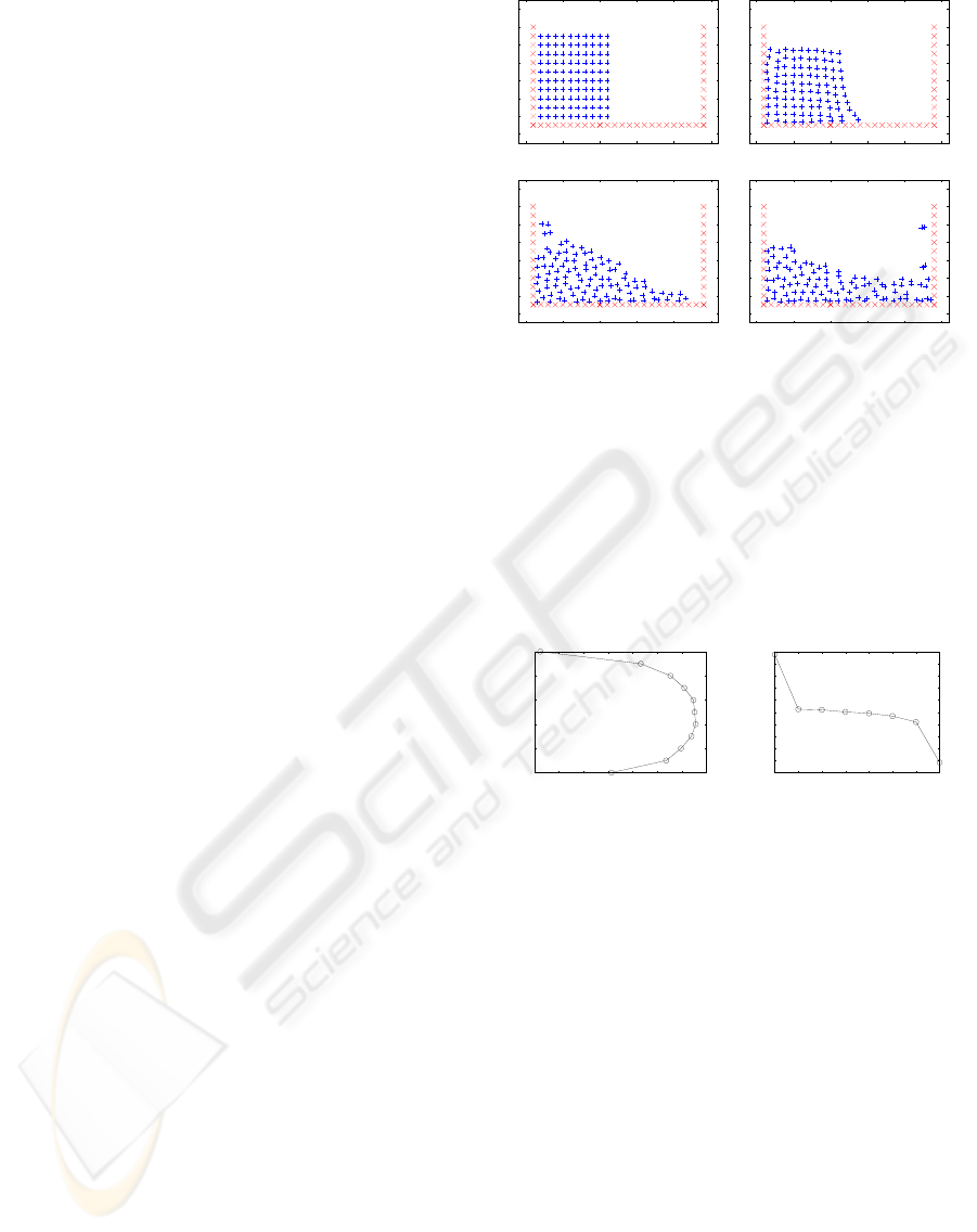
Fig. 1(a), we can see the initial state of the dam. The

working space is made up with the static particles

marked as “×”. The set of particles marked with “+”

form the incompressible ﬂuid. A border to the right of

the ﬂuid (the dam’s border) is removed at time t

. All

ﬂuid’s particles suffer a gravity force. In Fig. 1(b)-

(d) we can see the carried simulation. The simulation

works as expected, and it is similar to the showed in

(Monaghan, 1994).

The second experiment uses compliant simplex

meshes surfaces to model a tube where an incom-

pressible ﬂuid is running and the surface of a de-

formable sphere is placed inside the moving ﬂuid.

0.2

0.4

0.6

0.8

1.2

1.4

0 0.5 1 1.5 2 2.5

(a) t = 0 sec

0.2

0.4

0.6

0.8

1.2

1.4

0 0.5 1 1.5 2 2.5

(b) t = 0.1562 sec

0.2

0.4

0.6

0.8

1.2

1.4

0 0.5 1 1.5 2 2.5

0.2

0.4

0.6

0.8

1.2

1.4

0 0.5 1 1.5 2 2.5

(d) t = 0.4587 sec

Figure 1: Simulation of a dam’s rupture.

The ﬂuid moves by the action of an horizontal force

equal to the gravity force. It is difﬁcult to check by

visualization that the simulation is running ok in this

scenario. Thus, values along the ﬂuid are taken: the

average particle velocity through a transverse tubes’

section, and the average pressure through longitudi-

nal tubes’ sections. These values are shown on Fig. 2,

and we can see that simulation’s results are correct.

5 6 7 8 9 10 11 12

Transverse tubes’ sections

Velocity (m/s)

-5000

-4000

-3000

-2000

-1000

1000

2000

3000

4000

5000

1 2 3 4 5 6 7 8

Pressure (Pa)

Longitudinal tubes’ sections

Figure 2: Left curve shows the variation of the mean ve-

locity (horizontal axis) taken at a transverse section of the

tube (vertical axis). Right curve shows the average pressure

(horizontal axis) along the tube (horizontal axis).

Finally, in Fig. 3, we see several views of the sim-

ulation of the deformable sphere inside the ﬂuid. The

deformable surface takes the form of an ovoid, as it is

expected.

5 CONCLUSIONS

We developed a ﬂuid dynamics simulator based in the

Smooth Particle Hydrodynamics method plus the use

of compliant bodies modeled with simplex meshes.

The interface interaction has been modeled by orthog-

onal forces produced by each particle colliding with

the surface and simple models of 2

order compliant

deformation and Coulomb friction.

We can simulated containers or deformable ob-

jects contact with slightly compressible ﬂuids. Our

ICINCO 2009 - 6th International Conference on Informatics in Control, Automation and Robotics

272

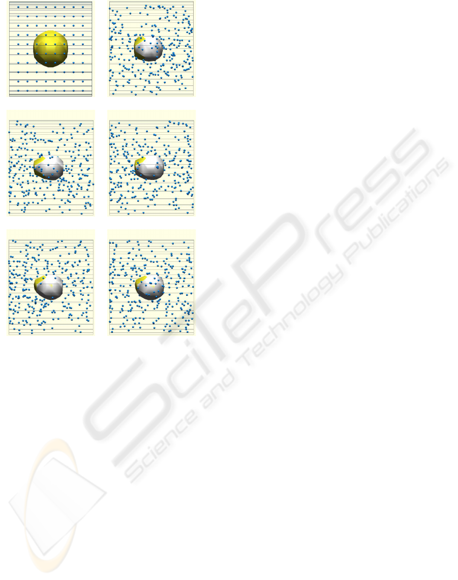
t = 0 sec t = 0.33 sec

t = 0.66 sec t = 0.99 sec

t = 1.98 sec t = 2.31 sec

Figure 3: Simulation of a deformable sphere immerse in a

ﬂuid contained within a tube.

simulator uses a simpliﬁed model of a compliant body

that allows fast computations. Our simulator can be

used in visualization of a real phenomena like to cut a

vein and to show how the blood ﬂuids.

We showed bidimensional simulations of the rup-

ture of a dam and a three-dimensional simulation of a

compliant sphere completely immersed in a running

incompressible ﬂuid inside a tube. The results simu-

late qualitative behaviors of the proved systems.

We are convinced that our method can be used as

a ﬁrst approximation, or to show graphically the be-

havior, of partial immersed bodies on compressible or

incompressible ﬂuids, like ships or submarines at the

see surface.

Also, the forces produced in immersed complex

mechanism, like robot arms attached to a ROV (Re-

motely Operated Vehicle) can be better understood if

more accurate hydrodynamical damping models can

be obtained. This method can be a good approach to

this end.

Finally, some work has to be done yet to reduce

the computational cost when a complex deformable

model is used, in order to obtain real time simulations.

ACKNOWLEDGEMENTS

This work has been partially supported by project

SEP-CONACyT 80965, M

exico.

REFERENCES

Chen, S., Johnson, D. B., and Raad, P. (1995). Velocity

boundary conditions for the simulation of free surface

ﬂuid ﬂow. Journal of Computational Physics, Volume

116(Issue 2, February):262–276.

chuan Bai, Y., Xu, D., and q. LU, D. (2007). Numerical sim-

ulation of two-dimensional dam-break ﬂows in curved

channels. Journal of Hydrodynamics, Ser. B, Volume

19(6):726–735.

Eddy, P., Natarajan, A., and Dhaniyala, S. (2006). Subisoki-

netic sampling characteristics of high speed aircraft

inlets: A new cfd-based correlation considering in-

let geometries. Journal of Aerosol Science, Volume

37(Issue 12, December):1853–1870.

Flores, J. R. and de la Fraga, L. (2004). Basic three-

dimensional objects constructed with simplex meshes.

In First International Conference on Electrical and

Electronics Engineering, pages 166–171. IEEE Pres.

Monaghan, J. and Lattanzio, J. (1985). A reﬁned method

for astrophysical problems. Astron. Astrophysics,

149:135–143.

Monaghan, J. J. (1994). Simulating free surface ﬂows with

sph. Journal of Computational Physics, 110:399–406.

Monaghan, J. J. (2005). Smoothed particle hydrodynamics.

Rep. Prog. Phys., 68:1703–1759.

erea, S. A., Gonz

alez, F. F., and Iglesias, A. S. (2005). Uti-

lizaci

on del m

etodo sph en la simulaci

on del sloshing.

Technical Report No. 822, Universidad de la Rioja.

Streeter, V. L. and Wylie, E. B. (1988). Fluid Mechanics.

Mc. Graw Hill.

Tai, C. H., Liew, K. M., and Zhao, Y. (2007). Numer-

ical simulation of 3d ﬂuid-structure interaction ﬂow

using an immersed object method with overlapping

grids. Computers & Structures, Volume 85(Issues 11-

14, June-July):749–762.

Trejo, C. R. and de la Fraga, L. G. (2005). Animation of de-

formable objects built with simplex meshes. In Second

International Conference on Electrical and Electron-

ics Engineering, pages 36–39. IEEE Pres.

van den Bergen, G. (2004). Collision Detection in Interac-

tive 3D Environments. Morgan Kaufmann.

EFFICIENT SIMULATION OF THE FLUID-STRUCTURE INTERFACE

273