MULTIOBJECTIVE GA-FUZZY LOGIC CONTROLLER
Applied to a pH Reactor
Orlando Reyes
Universidad Simón Bolivar, FEI, Dpto. De Tecnología Industrial, Calle Unibolivar, Baruta, Caracas, Venezuela
Gustavo Sánchez, Miguel Strefezza
Universidad Simón Bolivar, MYS, Dpto. De Procesos y Sistemas, Calle Unibolivar, Baruta, Caracas, Venezuela
Keywords: Genetic Algorithm, Multi-objective Optimization, Fuzzy Logic Controller.
Abstract: A Takagi-Sugeno (T-S) Fuzzy Logic Controller (FLC) is tuned using the algorithm NSGA-II. The proposed
method eliminates laborious design steps such as tuning of membership functions and conclusion table
parameters. An object approach representation is used to build an adequate FLC representation. Object is an
individual abstraction in order to improve crossover a mutation operators. The Genetic Algorithm
optimization is carry out over signal response performance parameters, in this work: settling time, rise time,
overshoot and steady state error. Experiments show how the algorithm reached good response of some
individuals in solution set, typically called Pareto frontier.
1 INTRODUCTION
pH control is a difficult benchmark problem due to
the nonlinearity and sensibility near the neutral
point. Control engineers would like to keep a
desirable set-point, rejecting disturbances and
tracking a reference signal.
FLC tuned via Genetic Algorithm (GA) to
control a pH reactor have shown good results in the
unconstrained case. In (Reyes et al, 2008) an object
approach was proposed to obtain the FLC
parameters, optimizing a scalar objective function
based on the loop error. The authors have also used
the sum of Rise time (Rt), Settling time (St),
Overshoot (Os) and Steady state error (Sse) as a
fitness function.
The indicators Rt, St, Os and Sse measure the
performance of a system response and could be in
possible conflict. If we try to minimize one, another
or the rest of metrics could increase. Real problems
involve more than one objective. Multiobjective
evolutionary techniques try to find the Pareto
frontier in the objective space (Coello, 2004), and
the control designer has to choose the best trade-off
for a given application.
2 MOEA
A multiobjective problem seeks to optimize the
components of a vector-valued objective function.
Unlike the single objective optimization the solution
to this problem is not a single point, but a family of
points know as the Pareto-optimal set (Tamaki et al,
1996). A multiobjective problem state can be stated
as:
Min f(x) = {f
1
(x),…….,f
i
(x),…….,f
n
(x)}
s.t. a x ∈ D
D = { x ∈ R
n
: g
j
(x) ≤ 0, j = 1,……., J;
h
k
(x) = 0, k = 1,......., K }
(1)
Several MOEAs have been proposed to solve
problem (1). In this work we propose to use the Non
dominated Search Genetic Algorithm (NSGA-II). It
initiates with a random population in the search
space, process follow assigning a particular rank to
the sequential Pareto surfaces generated plotting f
i
(x)
in the objectives space. After ranking assigned to
every individual other important parameter called
crowding distance tells how population density is or
individuals are scattered in objective space in a
particular Pareto frontier. The tournament process
chooses the best individuals and after a default
384
Reyes O., Sánchez G. and Strefezza M. (2009).
MULTIOBJECTIVE GA-FUZZY LOGIC CONTROLLER - Applied to a pH Reactor.
In Proceedings of the 6th International Conference on Informatics in Control, Automation and Robotics - Intelligent Control Systems and Optimization,
pages 384-389
DOI: 10.5220/0002210103840389
Copyright
c
 SciTePress

number of generations the algorithm stops. NSGAII
gives a set of solutions or Pareto surface.
Researchers use it if objectives to be optimized are
in conflict, thus no best or unique solution exist like
in a Simple Genetic Algorithm where a unique
solution is achieved.
3 CONTROLLER
Next, a briefing about Fuzzy Logic (FL), GA and
MOEA applied to this particular problem is
presented.
3.1 Fuzzy Logic
The Fuzzy Logic concept was proposed in a seminal
paper written in 1965 by Lofti A. Zadeh. One of the
first Fuzzy Logic Controlles (FLCs) was developed
by (Mandani & Assilian, 1975), attempting control
the speed of a steam engine.
An important issue in FLC design is searching
for adequate and if possible good parameters for
both membership functions and conclusion tables.
Heuristic techniques are useful to perform this task.
A FLC consists of a rule set that, in a linguistic
manner, tells how the system must work. The output
of the FLC will be the control action. Linguistic
rules are constructed like statements, with cause and
consequences, as follows:
IF cause_1 AND cause_2 THEN
consequence_1 AND consequence_2
In this work the defuzzification process is carried
out following the Takagi-Sugeno (T-S) method of
order cero, with five membership functions for each
input, and twenty five rules. Because is easy to
program and is faster than Mamdani method. The
FLC output is calculated using the weighted
averaging defuzzification method (see eq. 2).
,
*
j
ij
i
j
C
CF
α
α
=
∑
∑
(2)
where:
C
i,j
: conclusion i , rule j; α
j
: activation degree of
rule j;
CF
i
: defuzzificated (crisp) value.
An extended FLC review, presented in (Gang
Feng, 2006), gives the reader a clue of their broad
application.
Rules are created with all possible combinations
between Error and Derror fuzzy values. NB:
Negative Big, NS: Negative Small, Z: Zero, PS:
Positive Small, PB: Positive Big.
IF Error is NB AND Derror is PB THEN Ci,1
: : : : : : : : : : :
IF Error is PB AND Derror is NB THEN Ci,25
Next table show how to construct the rules.
Table 1: Rule table, i = 1 affects valve of acid, i = 2
otherwise.
Error
Derror
NB NS Z PS PB
PB C
i,1
C
i,2
C
i,3
C
i,4
C
i,5
PS C
i,6
C
i,7
C
i,8
C
i,9
C
i,10
Z C
i,11
C
i,12
C
i,13
C
i,14
C
i,15
NS C
i,16
C
i,17
C
i,18
C
i,19
C
i,20
NB C
i,21
C
i,22
C
i,23
C
i,24
C
i,25
Defuzfication is done calculating CF1:
conclusion at flow 1 and CF2: conclusion at flow 2,
with the equation 2. Where α
j
is the max value
between both membership degree Error and Derror
at the FLC input.
3.2 Genetic Algorithm
A Genetic Algorithm (Holland, 1975), (Golberg,
1953) is an iterative stochastic optimization process
based in how the nature selects the best individual to
survive within a given environment. They are now
accepted by both the optimization and control
communities to solve problems for which classical
methods (i.e mathematical programming) can not be
used or are not efficient enough. A GA starts with a
scattered random population in a bounded space. An
adaptation (or fitness) value is assigned to every
individual. Fitness will be used to give a selection
probability for crossover, survivor or mutation
operations. The choice of the best individuals for
crossover will give good “chromosomes” to
children. Mutation prevents premature convergence
relocating individuals. The process is iterated with
the hope to obtain better individuals when algorithm
stops.
3.3 NSGAII Procedure
Multiobjective problem (see eq. 1) start determining
searching space and spreading a randomly
population in it. Every individual is a FLC who’s
chromosomes are defined with membership
functions and conclusion tables parameters. In
simulation, individuals have it fitness vector
composed of {Rt, St, Os, Sse} (eq. 3), those are
objective space dimensions in where the individual
“adaptation” is plotted.
MULTIOBJECTIVE GA-FUZZY LOGIC CONTROLLER - Applied to a pH Reactor
385

Min f(x) = {Rt(x), St(x), Os(x), Sse(x)}
s.t. a x ∈ D
D = { x ∈ R
n
}
(3)
Where x are membership functions and conclusion
table parameters.
Individuals of population in objective space have
its particular Rank (R) and crowding distance (cd).
Rank is equal to one if individual belongs to Pareto
Frontier (PF), later those are removed and the
sequential individuals continue whit rank two and so
on, this process discriminate several local PF. Rank
assignment is done by PF definition (Augusto et al,
2006), consider two solutions vectors x and y, x is
contained in the PF if.
⎪
⎩
⎪
⎨
⎧
<∈∃
≤∈∀
)()(:,...,2,1
)()(:,...,2,1
yfxfkj
and
yfxfki
ij
ii
(4)
In the case of (4) x dominates y in the R
k
objective
space and have Rank one.
Crowding distance is the distance between one
individual and two near it in the same PF (see eq. 5).
()
∑∑
=
=
=
=
−=
mp
p
nc
c
cicpi
XXcd
11
2
(5)
Where c is an objective space axis and n are the
number of the objectives; p is a particular point and
m are the total points in the same Pareto Frontier; i is
the individual.
Binary selection is carry out and tournament is
done first by Rank. individuals with minor Rank are
preferred, if both have equal R, cd is taken into
account, mayor cd wins the tournament to preserve
population diversity, two individuals are then
selected by this process for crossover and mutation.
Simulated binary crossover (Deb & Agrawal,
1995) makes information interchange, and to avoid
premature convergence polynomial mutation works
well (see eq. 6).
(
)
k
l
k
u
kkk
pppc δ −+=
(6)
where k is the vector k-component, c is the child, p
the parent δ an uniform random number u and l are
the upper and lower bounds in the search space.
New and old population are joined and selected via
tournament to conform the new generation, and then
survivors could appear. The process is repeated until
reach the maximum number of iterations.
In a previous work, population of the Initial
Individuals where created with restrictions in
membership functions (Reyes et al, 2008) in hope of
avoid overlapping or empty space but no restrictions
where imposed while NSGAII was running, thus
membership functions at the end shown empty space
in discourse universe, overlapping or both mixed
cases (Fig. 2,3).
4 PH REACTOR
The equations for the pH dynamic were developed
in (McAvoy et al, 1975). The main issue is to keep
the process around the neutral point, where the
system is very sensitive and highly non linear, then
pH control is regarded as a benchmark problem,
especially when the reference signal change from
pH=7 to a mayor value nearby. The interested reader
can easily verify this fact by the construction of the
neutralization or titration curve (TC). An
experimental method to obtain the TC is based on
holding the base concentration constant, slowly
adding the acid and then plotting the pH versus the
acid concentration. Three operating zones are
commonly considered: low, medium, high (see Fig
1).
pH is usually controlled by the mixture of two
solutions with different concentrations, one basic
and other acid. In this work, we validated our
SIMULINK® model by comparing the resulting TC
with the one presented in (Zhang, 2001).
0 0.02 0.04 0.06 0.08 0.1 0.12 0.14 0.16 0.18 0.2
4
5
6
7
8
9
10
11
12
13
acid flow cc/m in
pH
-:C2= 0.05 m oles/l; --:C2 = 0.04 m oles/l; ..:C 2 = 0.06 m oles/l
Figure 1: Titration curve, zones low, medium, high, pH
approximately 0~6, 6~11.5, 11.5~14, respectively.
The neutralization process takes place within a
Continuous Stirred Tank Reactor (CSTR). There are
two flows to the CSTR. One is acetic acid of
concentration C
1
at flow rate F
1
, and the other is
sodium hydroxide of concentration C
2
at flow rate
F
2
.
The mathematical equations of the CSTR are
shown in eq’s 7-12.
Table 2 shows the parameters and model variables.
ICINCO 2009 - 6th International Conference on Informatics in Control, Automation and Robotics
386

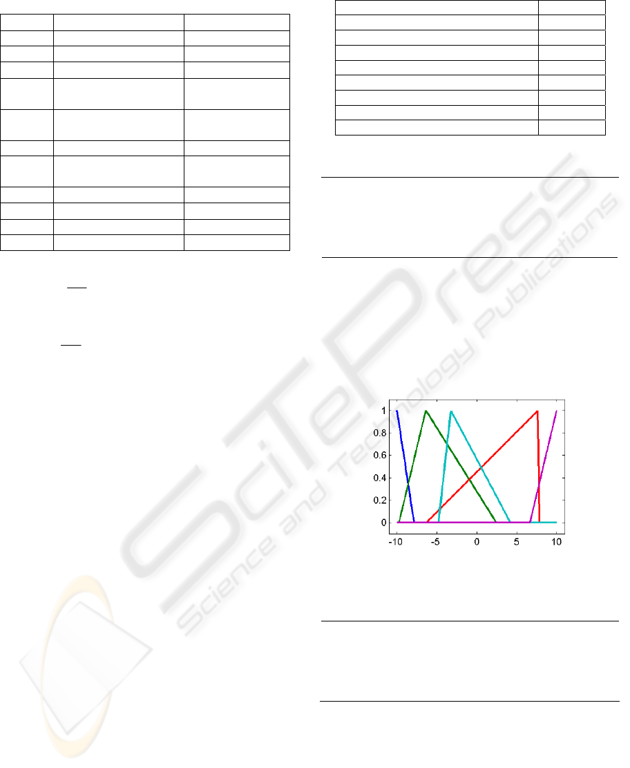
Table 2: Description and values for parameters and
variables.
Name Description Value
V Volume of tank 1 L
F
1
Flow rate of acid 0.081 L/min
F
2
Flow rate of base 0.512 L/min
C
1
Concentration of acid in
F1
0.32 mol/L
C
2
Concentration of acid in
F2
0.05005 mol/L
K
a
Acid equilibrium constant 1.8 X 10
-5
K
w
Water equilibrium
constant
1.0 X 10
-14
[H
+
] Hydrogen ion
-
[HAC] Acetic acid
-
[AC
-
] Acetate ion
-
[NA
+
] Sodium ion
-
11 1 2
()
d
VFCFF
dt
ξ
ξ
=−+
(7)
ς
ς
)(
2122
FFCF
dt
d
V +−=
(8)
[] []
(){} []
0
)(
23
=−−−
+++
+
++
awwa
a
KKHKK
HKH
ξς
ς
(9)
][log
10
+
= HpH
(10)
][][
−
+= ACHAC ξ
(11)
][
+
= NA ς
(12)
5 EXPERIMENT RESULTS
The experiment was done using MATLAB® and
SIMULINK®, starting parameters are shown in
table 3, they where defined by trial and error of
several experiments.
Following results where obtained from PF set for the
individual with minimum Sse (see Table 4). After
algorithm run designer choose what is more
convenient as desire system response, other values
could be refined if minimum of more than one
objective if required.
Table 3: Input parameters to the NSGAII.
Parameter Value
Generations 25
Individuals 30
Crossover probability 0.8
Mutation Probability 0.01
Error Domain [-10 10]
Rate of error Domain [-10 10]
Conclusion Domain at inlet 1 [0 7]
Conclusion Domain at inlet 2 [0 7]
Values of membership functions parameters for
error
-10.00 -5.95
-9.75 -6.39 2.42
-6.31 7.65 7.80
-4.79 -3.25 4.20
5.84 10.00
Left trapeze
Triangle
“
“
Right trapeze
Figures 2 show the final distribution of the error
membership functions, in where overlapping appear
in absent of restrictions while NSGAII was running.
Figures 3 show the final rate of error distribution
membership functions, in where empty space and
overlapping appear in absent of restrictions while
NSGAII was running.
Figure 2: Error membership functions.
Values of membership functions parameters for rate
of error
-7.00 -5.10
-6.87 -5.86 -3.21
0.67 0.92 2.77
-0.15 5.14 6.73
5.80 7.00
Left trapeze
Triangle
“
“
Right trapeze
MULTIOBJECTIVE GA-FUZZY LOGIC CONTROLLER - Applied to a pH Reactor
387

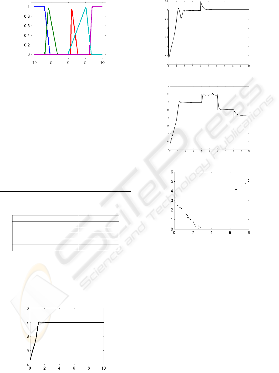
Figure 3: Rate of error membership functions.
Consequence values (according to Table 1) are used
in the FLC to get and adequate system response.
Consequence matrix, flow 1
6.23 6.98 6.17 5.17 4.39
5.35 4.93 2.46 4.25 2.48
0.97 1.04 2.95 3.61 0.18
3.01 6.20 6.22 5.31 2.72
0.48 2.73 0.84 1.14 6.48
Consequence matrix, flow 2
5.40 0.08 2.01 5.63 5.94
1.98 0.11 3.63 5.45 5.14
5.82 5.97 6.89 2.90 6.59
6.23 0.05 0.70 2.40 0.15
6.31 3.81 4.43 0.44 4.80
Table 4: Objectives to the individual with minimum Sse
NSGAII.
Objective Value
Settling time 2.0511
Undershoot 2.5918
Overshoot 0.1158
Rise Time 3.4483e-004
Steady State Error 0.0217
System response with FLC parameters at the final of
the NSGAII run do its job following reference signal
and disturbance rejection near neutral point (Fig. 4-
6).
Os and Sse where the only objectives in conflict as
show in Fig 7. against other objectives combined
and that’s why there aren’t shown here.
Figure 4: System response pH vs time.
Figure 5: Disturbance Rejection.
Figure 6: Signal tracking.
Figure 7: Space Os vs Sse.
6 CONCLUSIONS
Multiobjective Evolutionary Algorithms in the case
of NSGAII is an excellent tool to find FLC
membership functions and conclusion table
parameters, especially is control designer wants to
refine one objective on case depending. The method
gives a population of FLC to choose a desired one,
additionally shows what objectives are opposed.
Parameters in table 3 are subject of discussion with
more intensive run of the whole algorithm.
The algorithm is very slow, every individual of
population must be simulated also fitness assigned,
and is necessary a lot of computer resource but is
achieved of line.
ICINCO 2009 - 6th International Conference on Informatics in Control, Automation and Robotics
388

7 FUTURE WORK
Basic restrictions would be imposed to obtain more
homogeneous membership functions distribution,
avoiding overlapping and empty space in discourse
universe in membership functions.
Program Mamdani method applying restrictions in
consequence and compare difference in response.
Algorithm stop criteria must be implemented to
compare it with other MOEA in order to establish
performance metrics.
REFERENCES
Reyes, O., Sanchez, G., Strefezza, Miguel, 2008. Usign
Genetic Algorithms to design a Fuzzy Logic
Controller for a pH Reactor: an Object Approach.
“IASTED International conference, Quebec City,
Canada Control and Applications (CA 2008) May 26-
28”, Proceedings of the xxx conference IASTED.
http://www.actapress.com/Abstract.aspx?paperId=336
09
L. A. Zadeh. Fuzzy Sets. 1965. Information and Control
Vol 8. 338-353.
E. H. Mamdani and Assilian. 1975. An Experiment In
Linguistic Synthesis with a Fuzzy Logic Controller.
Int. Man Mach Stud Vol. 7. 1-13.
Moore, R., Lopes, J., 1999. Paper templates. In
TEMPLATE’06, 1st International Conference on
Template Production. INSTICC Press.
Smith, J., 1998. The book, The publishing company.
London, 2
nd
edition.
E. H. Mandani and S. Assilian. 1975. An Experiment In
Linguistic Synthesis with a Fuzzy Logic Controller,
Int. J. Man Mach. Stud. Vol. 7. 1-13.
Holland, J. Adaptation in Natural and Artificial Systems.
1975. University of Michigan Press, Ann Arbor.
David E. Golberg, Genetic Algorithms in Search
Optimization & Machine Learning. 1953.Addison
Wesley Longman Inc.
Gang Feng. 2006. A Survey on Analysis and design of
Model-Based Fuzzy Control Systems. IEEE
Transactions on Fuzzy Systems,14(5).
McAvoy, T. J.; Hsu, E.; Lowenthal, S. 1975. Dynamics of
pH in a Controled Stirred Tank Reactor. Ind. Eng.
Chem. Process Des. Dev. 11. 68 –70.
Zhang, J. 2001.A Nonlinear Gain Scheduling Control
Strategy Based on Neuro-Fuzzy Networks. Ind. Eng.
Chem. Res. 40. 3164 –3170.
Carlos A. Coello Coello. 2004. Recent Trends in
Evolutionary Multiobjective Optimization.
Evolutionary Multiobjective Optimization Theoretical
Advances and Applications. Springer. ISBN 1-85233-
787-7.
Deb, K.; Agrawal, S.; Pratab, A. & Meyarivan, T. 2000. A
Fast Elitist Non-Dominated Sorting Genetic Algorithm
for Multiobjective Optimization: NSGAII.
Proceedings of Parallel Problem Solving From Nature
VI Conference, pp 849-858.
O.B. Augusto, S. Rabeau, Ph. De’pince, F. Bennis. 2006.
Multi-objective genetic algorithms: a way to improve
the convergence rate. Engineering Applications of
Artificial Intelligence 19, 501–510
H. Tamaki, H. Kita, and S. Kobayashi. 1996. Multi-
objective optimization by Genetic Algorithms: A
review. IEEE Proc. Int. Conf. Evolutionary
Computation, 517–522
MULTIOBJECTIVE GA-FUZZY LOGIC CONTROLLER - Applied to a pH Reactor
389