SIMPLE DESIGN OF THE STATE OBSERVER FOR LINEAR
TIME-VARYING SYSTEMS
Yasuhiko Mutoh
Department of Applied Science and Engineering, Sophia University, 7-1, Kioicho, Chiyoda-ku, Tokyo, Japan
Keywords:
Pole placement, State observer, Linear time-varying system.
Abstract:
A simple design method of the Luenberger observer for linear time-varying systems is proposed in this paper.
The paper first propose the simple calculation method to derive the pole placement feedback gain vector for
linear time-varying systems. For this purpose, it is shown that the pole placement controller can be derived
simply by finding some particular ”output signal” such that the relative degree from the input to this output is
equal to the order of the system. Using this fact, the feedback gain vector can be calculated directly from plant
parameters without transforming the system into any standard form. Then, this method is applied to the design
of the observer, i.e., because of the duality of linear time-varying system, the state observer can be derived by
un-stabilization of the state error equation.
1 INTRODUCTION
The design of the pole placement and the state ob-
server for linear time-varying systems is well estab-
lished problem. As for the linear time-invariant case,
if the system is controllable, the pole placement con-
troller can be designed, and, if observable, the state
observer can be designed. However, many of those
design method need a complicated calculation proce-
dure. In this paper, a simple design method of the
Luenberger observer for linear time varying systems
is proposed.
Since, the observer design problem is the dual
problem of the pole placement, simplified calculation
method to derive the pole placement feedback gain
vector for linear time-varying systems should be con-
sidered first. Usually, the pole placement procedure
needs the change of variable to the Flobenius standard
form, and hence, is very complicated (e.g., Michael
Val´aˇsek and Nejat Olgac¸). To simplify this procedure,
it will be shown that the pole placement controller can
be derived simply by finding some particular ”output
signals” such that the relative degree from the input
to this output is equal to the order of the system. This
is motivated from the fact that the input-output lin-
earization of a certain type of nonlinear systems is
equivalent to the entire state linearization, if the rela-
tive degree of the system is equal to the system order.
Using this fact, the feedback gain vector can be cal-
culated directly from plant parameters without trans-
forming the system into any standard form.
Because of the duality of the linear time-varying
system, the state observer can be derived by unsta-
bilizing the state error eqation. This implies that the
simplified pole placement technique can be applied to
the design of the state observer for linear time-varying
systems to obtain simpler design method than existing
methods from the point of view of the calculational
compexity.
In the sequel, the simple pole placement technique
is proposed in Section 2, and then, this method is used
to the observer design problem in Section 3.
2 POLE PLACEMENT OF
LINEAR TIME-VARYING
SYSTEMS
Consider the following linear time-varying system
with a single input.
˙x = A(t)x+ b(t)u (1)
Here, x ∈ R
n
and u ∈ R
1
are the state variable and
the input signal respectively. A(t) ∈ R
n×n
and b(t) ∈
R
n
are time-varying parameter matrices. The problem
is to find the state feedback
u = k
T
(t)x (2)
225
Mutoh Y. (2009).
SIMPLE DESIGN OF THE STATE OBSERVER FOR LINEAR TIME-VARYING SYSTEMS.
In Proceedings of the 6th International Conference on Informatics in Control, Automation and Robotics - Signal Processing, Systems Modeling and
Control, pages 225-229
DOI: 10.5220/0002206002250229
Copyright
c
 SciTePress

which makes the closed loop system equivalent to
the time invariant linear system with arbitrarily stable
poles.
Now, consider the problem of finding a new output
signal y(t) such that the relative degree from u to y is
n. Here, y(t) has the following form.
y(t) = c
T
(t)x(t) (3)
Then, the problem is to find a vector c(t) ∈ R
n
that
satisfies this condition.
Lemma 1. Let c
T
k
(t) be defined by the following
equation.
c
T
k
(t) = ˙c
T
k−1
(t) + c
T
k−1
(t)A(t), c
T
0
(t) = c
T
(t) (4)
The relative degree from u to y defined by (3) is n,
if and only if
c
T
0
(t)b(t) = c
T
1
(t)b(t) = ··· = c
T
n−2
(t)b(t) = 0
c
T
n−1
(t)b(t) = 1 (5)
(Here, c
T
n−1
(t)b(t) = 1 without loss of generality.)
Proof : By differentiating y successively using (5),
the following equations are obtained from (1) and (3).
y = c
T
(t)x
= c
T
0
(t)x
˙y =

˙c
T
(t) + c
T
(t)A(t)

x+ c
T
(t)b(t)u
= c
T
1
(t)x+ c
T
0
(t)b(t)u
= c
T
1
(t)x
¨y =

˙c
T
1
(t) + c
T
1
(t)A(t)

x+ c
T
1
(t)b(t)u
= c
T
2
(t)x+ c
T
1
(t)b(t)u
= c
T
2
(t)x (6)
.
.
.
y
(n−1)
= c
T
n−1
(t)x+ c
T
n−2
(t)b(t)u
= c
T
n−1
(t)x
y
(n)
= c
T
n
(t)x+ c
T
n−1
(t)b(t)u
= c
T
n
(t)x+ u
This implies that the relative degree from u to y is
n. ∇∇
Lemma 2. If c
T
(t) satisfies the condition that the rel-
ative degree from u to y is n, then we have the follow-
ing equation.
[c
T
0
(t)b(t), c
T
1
(t)b(t), ··· , c
T
n−1
(t)b(t)]
= [c
T
(t)b
0
(t), c
T
(t)b
1
(t), ··· , c
T
(t)b
n−1
(t)]
(7)
where b
i
(t) is defined by
b
i
(t) = A(t)b
i−1
(t) −
˙
b
i−1
(t), b
0
(t) = b(t) (8)
Proof : First, the following is trivial.
c
T
0
(t)b(t) = c
T
(t)b(t) = c
T
(t)b
0
(t) (9)
From (5), we have
˙c
T
0
(t)b(t) = −c
T
0
(t)
˙
b(t) (10)
which implies
c
T
1
(t)b(t) = ˙c
T
0
(t)b(t) + c
T
0
(t)A(t)b(t)
= −c
T
0
(t)
˙
b(t) + c
T
0
(t)A(t)b(t)
= c
T
0
(t)b
1
(t)
= c
T
(t)b
1
(t) (11)
In a similar fashion, from (5) and (11), we have
˙c
T
0
(t)b
1
(t) = −c
T
0
(t)
˙
b
1
(t)
˙c
T
1
(t)b(t) = −c
T
1
(t)
˙
b(t) (12)
which implies
c
T
2
(t)b(t) = ˙c
T
1
(t)b(t) + c
T
1
(t)A(t)b(t)
= −c
T
1
(t)
˙
b(t) + c
T
1
(t)A(t)b(t)
= c
T
1
(t)b
1
(t)
= ˙c
T
0
(t)b
1
(t) + c
T
0
(t)A(t)b
1
(t)
= −c
T
0
(t)
˙
b
1
(t) + c
T
0
(t)A(t)b
1
(t)
= c
T
0
(t)b
2
(t)
= c
T
(t)b
2
(t) (13)
By continuing the same process, (7) is derived. ∇∇
From Lemma 2, (5) implies
[c
T
0
(t)b(t), c
T
1
(t)b(t), ··· , c
T
n−1
(t)b(t)]
= [c
T
(t)b
0
(t), c
T
(t)b
1
(t), · ·· , c
T
(t)b
n−1
(t)]
= c
T
(t)[b
0
(t), b
1
(t), · ·· , b
n−1
(t)]
= c
T
(t)U
c
(t)
= [0, 0, · · · , 1] (14)
Here,
U
c
(t) = [b
0
(t), b
1
(t), · ·· , b
n−1
(t)] (15)
where, U
c
(t) the controllability matrix for linear time-
varying system (1). If U
c
(t) is nonsingular for all t ∈
[0, ∞), the system is said to be controllable. Hence,
we have the following Theorem.
Theorem 1. If the system (1) is controllable, there
exists a vector c(t) such that the relative degree from
u to y = c
T
(t)x is n. And, such a vector, c(t) is given
by
c
T
(t) = [0, 0, ··· , 1]U
−1
c
(t) (16)
∇∇
The next step is to derive the state feedback for the
arbitrary pole placement. Let q(p) be a desired stable
polynomial of the differential operator, p, i.e.,
q(p) = p
n
+ α
n−1
p
n−1
+ ··· + α
0
(17)
ICINCO 2009 - 6th International Conference on Informatics in Control, Automation and Robotics
226

By multiplying y
(i)
by α
i
(i = 0, ··· , n − 1) and then
summing them up, the following equation is obtained,
using (5) and (6).
q(p)y = d
T
(t)x+ u (18)
where d(t) ∈ R
n
is defined by the following.
d
T
(t) = [α
0
, α
1
, ·· · , α
n−1
, 1]







c
T
0
(t)
c
T
1
(t)
.
.
.
c
T
n−1
(t)
c
T
n
(t)







(19)
Hence, the state feedback,
u = −d
T
(t)x+ r (20)
makes the closed loop system as follows.
q(p)y = r (21)
where r is an external input signal. This method is
regarded as an extension of Ackermann’s pole place-
ment method to the time-varying case.
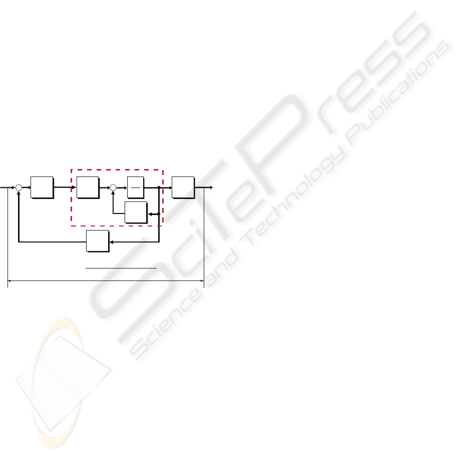
M
-
1
s
M
M M
M
M
Λ
-1
b
c
A
D
(t)
(t)
v
y
u
(t)
(t)
(t)
1
1 0
1
n n
n
s sα α
−
−
+ + +⋯
Figure 1: Blockdiagram of Pole Placement for a Linear
Time-Varying System.
This control system can be summarized as fol-
lows. The given system is
˙x = A(t)x+ b(t)u (22)
and, using (16) and (19), the state feedback for the
pole placement is given by
u = −d
T
(t)x. (23)
Then, the closed loop system becomes
˙x = (A(t) − b(t)d
T
(t))x. (24)
At the same time, we have (21) as another rep-
resentation of the closed loop system. This can be
explained as follows.
Let T(t) be the time varying matrix defined by
T(t) =





c
0
(t)
T
c
1
(t)
T
.
.
.
c
T
n−1
(t)





(25)
and define the new state variable w by
x = T(t)w, w =





y(t)
˙y(t)
.
.
.
y
(n−1)
(t)





(26)
Theorem 2. If the system (1) is controllable, then, the
matrix for the change of variable, T(t), given by (25)
is nonsingular for all t. ∇∇
This theorem can be proved by simple calculation
as for the time invariant case.
Then, (24) is transformed into
˙w = {T(t)(A(t) − b(t)d
T
(t))T
−1
(t) − T(t)
˙
T
−1
(t)}w
=






0 1 ··· 0
.
.
.
.
.
.
.
.
.
.
.
. 1
−α
0
··· · ·· −α
n−1






w = A
∗
w (27)
This implies that the closed loop system is equiv-
alent to the time invariant linear system which has the
desired closed loop poles. (det(pI − A
∗
) = q(p))
3 STATE OBSERVER
In this section, we consider the design of the observer
for the following linear time-varying system.
˙x = A(t)x+ b(t)u
y = c
T
(t)x (28)
Here, y ∈ R is the output signal of this system. The
problem is to design the full order state observer of
(28). Consider the following system as a candidate of
the observer.
˙z = F(t)z+ b(t)u + h(t)y
= F(t)z+ b(t)u + h(t)c
T
(t)x (29)
where F(t) ∈ R
n×n
, and h(t) ∈ R
n
. Define the state
error e ∈ R
n
by
e = x− z (30)
Then, e satisfies the following error equation.
˙e = F(t)e+ (A(t) − F(t) − h(t)c
T
(t))x (31)
SIMPLE DESIGN OF THE STATE OBSERVER FOR LINEAR TIME-VARYING SYSTEMS
227

Hence, (29) is a state observer of (28) if F(t) and h(t)
satisfy the following condition.
F(t) = A(t) − h(t)c
T
(t) (32)
F(t) : arbitrarily stable matrix
Consider the pole placement control problem of
the following system.
˙x = −A
T
(t)x+ c(t)u (33)
From the property of the duality of the time varying
system, if the pair (A(t), c
T
(t)) is observable, the pair
(−A
T
(t), c(t)) is controllable. This implies that if the
system (28) is observable, there is a state feedback
for the arbitrary pole placement for the system (33).
Let (λ
1
, λ
2
, ·· · , λ
n
) be the set of desired stable closed
loop poles.
Suppose that
u = k
T
(t)x (34)
is the state feedback for (33) with the desired un-
stable closed loop poles, (−λ
1
, −λ
2
, ·· · , −λ
n
). The
closed loop system is
˙x = (−A
T
(t) + c(t)k
T
(t))x (35)
This implies that, using the appropriate change of
variable, x = P(t)w, (35) can be transformed into the
following time invariant system.
˙w = {P
−1
(t)(−A
T
(t) + c(t)k
T
(t))P(t)
−P
−1
(t)
˙
P(t)}w
= −F
∗T
w (36)
Here, the eigenvalues of −F
∗
are (−λ
1
, −λ
2
, ·· · ,
−λ
n
).
It is also well known that if the fundamental ma-
trices of (35) and its dual system,
˙x = (A(t) − k(t)c
T
(t))x (37)
are Φ(t, t
0
) and Ψ(t, t
0
), respectively, then,
Φ(t, t
0
) = Ψ
T
(t
0
, t). (38)
Furthermore, by the change of variable,
x = (P
T
(t))
−1
ξ (39)
(35) is transformed into
˙
ξ = (P
T
(A(t) − k(t)c
T
(t))(P
T
)
−1
− P
T
(
˙
P
T
)
−1
)ξ
= (P
T
(A(t) − k(t)c
T
(t))(P
T
)
−1
+
˙
P
T
(P
T
)
−1
)ξ
=

P
−1
(A
T
(t) − c(t)k
T
(t))P+ P
−1
˙
P

T
ξ
= F
∗
ξ (40)
Hence, by choosing
h(t) = k(t) (41)
(29) becomes the observer for (28), and the state error
equation becomes
˙e = F(t)e (42)
which is equivalent to (40). That is, if the system
(28) is observable, it is possible to design h(t) so that
the state estimation error equation is equivalent to the
time invariant homogeneous system which has the ar-
bitrary stable poles.
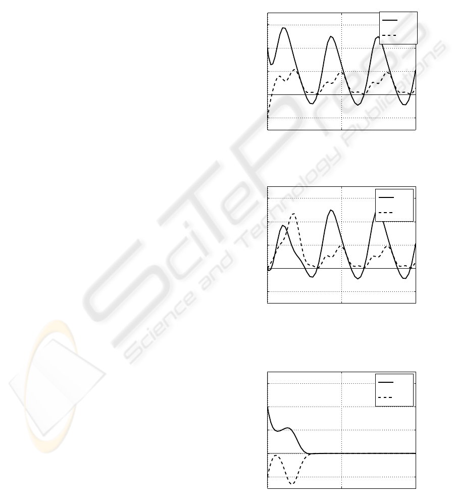
0 10 20
-1
0
1
2
3
x1
x2
Figure 2: Responce of the state variable (x) of the system.
0 10 20
-1
0
1
2
3
z1
z2
Figure 3: Responce of the state variable of the observer (z).
0 10 20
-1
0
1
2
3
e1
e2
Figure 4: Responce of the state error (e = x− z).
ICINCO 2009 - 6th International Conference on Informatics in Control, Automation and Robotics
228

Example 1. Consider the following system.
˙x = A(t)x+ b(t)u
y = c
T
(t)x (43)
where
A(t) =

−1, 1
−1+ sin2t − cost, −3+ cost

b(t) =

2+ sint
0

c
T
(t) =

2+ sin0.5t 0

(44)
This is a stable time-varying observable system. Fig.2
shows the response of the state variable of this system
with
u = sint (45)
The state observer is the following.
˙z = (A(t) − h(t)c
T
(t))z+ b(t)u+ h(t)y (46)
where we choose the desired observer poles as − 1
and −2. (The numerical details are omitted in this
draft paper.)
Fig.3 and 4 show the state variable of the observer
and the state error.
4 CONCLUSIONS
In this paper, one design method for the state observer
for linear time-varying systems is proposed. We first
proposed the simple calculation method for the pole
placement state feedback gain for liner time-varying
system. Feedback gain can be derived directly from
the plant parameter without the transformation into
any standard form.
In this method, since the transformation of the
given system into the Flobenius standard form is not
required, the design procedure is very simple. It was
shown that if the system is observable, then the state
observer can be obtained with arbitrarily stable ob-
server poles.
REFERENCES
Charles C. NguyenC Arbitrary eigenvalue assignments for
linear time-varying multivariable control systems. In-
ternational Journal of Control, 45-3, 1051–1057, 1987
Chi-Tsong ChenC Linear System Theory and Design (Third
edition). OXFORD UNIVERSITY PRESS, 1999
T. KailathC Linear Systems. Prentice-Hall, 1980
Michael Val´aˇsek, Nejat Olgac¸ Efficient Eigenvalue Assign-
ment for General Linear MIMO systems. Automatica,
31-11, 1605–1617, 1995
Michael Val´aˇsek, Nejat Olgac¸C Pole placement for linear
time-varying non-lexicographically fixed MIMO sys-
tems. Automatica, 35-1, 101–108, 1999
SIMPLE DESIGN OF THE STATE OBSERVER FOR LINEAR TIME-VARYING SYSTEMS
229