VEHICLE ACCELERATION PREDICTION
USING SPECIFIC ROAD CURVATURE POINTS
Aušra Vidugirienė, Andriejus Demčenko and Minija Tamošiūnaitė
Vytautas Magnus University, Vileikos st. 8, LT-44404 Kaunas, Lithuania
Keywords: Human-like driving, Intelligent driver’s assistance, Longitudinal control, Curve-based parameters.
Abstract: In the work vehicle acceleration prediction issue is discussed. Three types of parameters are used for
prediction system input: CAN-bus parameters – speed and curvature, derived speed parameters and newly
offered specific curve point parameters, denoting changes in a curve. The real road data was used for
predictions. Road curvature segments were divided into single and S-type curves. Acceleration was
predicted using artificial neural networks and look-up table. The look-up table method showed the best
results with newly offered specific curve parameters.
1 INTRODUCTION
Driving assistance systems are becoming a usual
component of modern cars. Here we are developing
an algorithm that could aid to driver's assistance on a
curved country road. One way to develop such
algorithms is through modelling driver's behaviour.
Once we have a model that predicts driver's
behaviour, we can compare actual behaviour with
the prediction, and warn the driver if there is
inconsistency.
In the field of driving action description several
clear-cut situations have been studied exhaustively:
lane following (Fenton, 1988; Mammar et al., 2006),
car following at a safe distance (Gipps, 1981;
Olstam et al., 2004), lane change (Gipps, 1986;
Salvucci et al., 2007). For lane following on a
curved road an extensive theory has been developed,
mainly based on control engineering approaches
(Hsu et al., 1998; Yuhara et al., 2001; Chen et al.,
2006; Mammar et al, 2006). Yet speed control (so
called longitudinal control), including speed on
curves, has only been studied extensively from a car
stability perspective (Jin et al., 2007; Hel et al.,
2007; Song, 2008). Alternatively, we focus on
predicting speed (or acceleration) profiles of
individual drivers, where they are performing not at
the limits of car possibilities, but rather in their
comfort-driving modes. Speed prediction of an
individual driver is a much more complicated
problem as compared to steering prediction, because
of much stronger influence of contextual
information, and less constraint for a driver in
choosing the actual speed profile. There are only
singular investigations concerning speed prediction
based on speed profiles of individual driver, e.g.
(Partouche et al., 2007), and success of such work
until now is quite limited.
In this study we apply learning techniques to
predict individual driver's acceleration on a curve.
Neural networks and look-up tables are employed
for prediction. Real road driving data is used, and
input parameters for driver's action prediction are
analyzed.
Relatively long real road data sequences are
required for predicting acceleration on a curve. This
is because speed control process has a wider time
scale than steering, i.e. for generating velocity
control the driver reacts rather to future events, like
upcoming curves, than immediate situations. E.g. it
was observed in this study that deceleration in front
of a curve starts 3-6 s or on some occasions even up
to 10 s in advance. Consequently, multiple curve
taking situations in the recordings are required to
derive the algorithm that predicts an expected
acceleration profile for a particular driver on a
particular curve. This makes the problem of speed
(or acceleration) prediction on a curve difficult to
address, especially when using real-road data.
147
VidugirienÄ
˚
U A., DemÄ enko A. and TamoÅ ˛aiÅ
´
nnaitÄ
˚
U M.
VEHICLE ACCELERATION PREDICTION USING SPECIFIC ROAD CURVATURE POINTS.
DOI: 10.5220/0002173401470152
In Proceedings of the 6th International Conference on Informatics in Control, Automation and Robotics (ICINCO 2009), page
ISBN: 978-989-674-000-9
Copyright
c
 2009 by SCITEPRESS – Science and Technology Publications, Lda. All rights reserved

2 DATA FOR ACCELERATION
PREDICTION
Two data sets were used for the study. The first data
set was collected during November-December,
2006. The second data set was collected in
December, 2007. Both data sets were obtained on
country roads nearby Lippstadt, Germany; at day
light, on a test car (Volkswagen Passat). In the data
set from 2006, ten recordings, approximately six
minutes length each were provided. Five of those
recordings were obtained on the same road, using
forward direction, and the other five were obtained
using backward direction. The recordings were
coming from two drivers: eight recordings of the
first driver, and two recordings of the second driver.
The second set of data (year 2007) consisted of six
recordings. Those recordings were obtained on a
different road as compared to the recordings from
the year 2006. The recordings were again obtained
in forward and backward directions, duration of ten
minutes each. This set of recordings was repeated
three times for three different drivers.
The test car control data were recorded using
CAN-bus with a sampling interval of 0.06 s. The
following signals were extracted from the CAN-bus
and used in the study:
 velocity v(t),
 acceleration a(t),
 curvature of the road c(t); curvature was
measured using a gyroscope installed in the
car.
3 METHODS
Curvature-based parameters combined with car
velocity were employed to predict driver's
acceleration. In this work gyroscopically measured
curvature was used, as a shortcut proceeding
towards further systems, where image processing or
digital map information will be used to obtain the
curvature in front of a car.
Neural networks and look-up tables were used as
function approximation means for prediction. For
neural network analysis a simple neural network
with one hidden layer was used. There were from
two to four neurons in the hidden layer, according to
the number of input parameters. Separate learning
data sets and test sets were employed. The average
of prediction error from ten initializations was
calculated to make results more reliable.
In the look-up table approach input parameter
values obtained at discrete time moments were
stored together with corresponding acceleration
signal value. The predictions were made as follows:
for the input parameter vector obtained at a specific
time moment mean squared error (MSE) was
calculated between that vector and every instance of
the look-up table. The predicted acceleration was
calculated as the mean of ten acceleration values,
with the smallest MSE to input parameters. In
addition, the acceleration signal was smoothed using
20 point moving average filter (corresponds to 1.2 s)
from the previous predictions.
As part of the input vector raw CAN-bus signals:
curvature and speed were used, but also a large set
of derived parameters was introduced.
Among the derived parameters we used
centrifugal acceleration (Hong et al, 2006):
R
v
a
c
2
=
(1)
where R denotes the curve radius, and v is the speed.
The centrifugal acceleration is considered to be a
parameter influencing driving comfort and possibly
driver’s actions (Hong et al, 2006).
We used speed differences S
d
=v(t)-v(t-Δt) over
several second intervals (Δt=0.5, 1.0, 1.5, 2.0, 2.5,
3.0 s) to account for previous acceleration or
deceleration actions. If a car decelerated, the speed
difference was negative, and if the car was
accelerating, the speed difference was positive.
For acceleration on a curve, features like the
distance to a start of a curve or the distance to the
end of a curve are important. We introduced a set of
curve shape based points (see Fig. 1), that later were
employed to derive features for acceleration
analysis. All the parameters’ notations are listed in
Table 1.
Table 1: Curve- and speed-derived parameters.
Parameter
class
Parameter Notation
CAN-bus
derived
parameters
Centrifugal acceleration CA
Speed difference
(now-Xs back)
SD-X
Single
curve
parameters
Start S
Start peak SP
End peak EP
End E
S-curve
parameters
S-curve start peak SSP
S-curve zero crossing S0
S-curve end peak SEP
ICINCO 2009 - 6th International Conference on Informatics in Control, Automation and Robotics
148

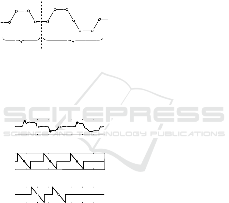
Two different curve shapes were analyzed in this
work:
 Single curve that has 4 specific points (start,
start peak, end peak and end; see Fig. 1a),
 S-shaped curve that has 7 specific points (start,
start peak, S start peak, S zero crossing, S end
peak, end peak and end; see Fig. 1b).
a
b
S
SP EP
E
S
SP SSP
S0
SEP
EP
E
Figure 1: Specific curve-based points’ scheme: a) single
curve with 4 specific points: start (S), start peak (SP), end
peak (EP) and end (E); b) S-shaped curve with 7 specific
points: start (S), start peak (SP), S start peak (SSP), S zero
crossing (S0), S end peak (SEP), end peak (EP) and end
(E).
The features were described as distances from
specific points. Examples of feature time series are
provided in Fig. 2.
x 10
-
3
road curve
1/R, 1/m
0 10 20
30
40 50 60 70 80
-100
0
"start peak" (SP) parameter
time, s
"end" (E) parameter
100
0
5
-5
01020
20 10
0
30
30
40
40
50
50
60
60
70
70
80
80
100
0
-100
time, s
time, s
a
b
c
Figure 2: Curvature (a) and features describing distances
to specific points on a curve (b and c). Features for the
points ‘Start peak’ and ‘End’ are shown. The points ‘Start
peak’ are marked by black points and the points ’End’ in
circles.
Before a specific point it is considered how
much time is left to that point, and after the point it
is pointed out how much time has passed since the
specific point had been passed. A feature is started
to be considered six seconds in advance before a
specific point is reached and the point is “forgotten”
six seconds after it has been passed. Before the point
a feature is positive, at the point it is zero, and after
the point it is negative.
An algorithm to derive feature values is as
follows: first, the specific curve point t
p
is
determined and the feature value for that discrete
time moment is set to zero. The feature values are
calculated by adding 1 or -1 to the previous value
when going through every discrete time step back
and forward respectively. The calculations end when
t
back
=t
p
-100 and t
forward
=t
p
+100 (100 discrete points
corresponds to 6 s according to the signal
discretization).
4 ACCELERATION PREDICTION
RESULTS
4.1 Acceleration Predictions using Raw
CAN-bus Signals
We used curvature c(t+Δ) where Δ = 4s (that is, four
seconds ahead), and speed v(t) to predict
acceleration one step forward. The training set was
composed of seven curve segments containing clear
acceleration-deceleration patterns, and we predicted
the segment that was not included into the learning
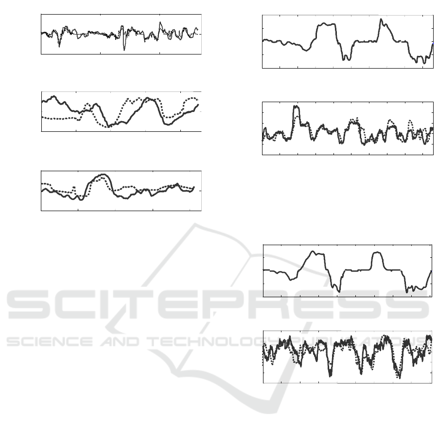
data set. Examples of predicted signals are presented
in Fig. 3.
As can be seen in the Fig. 3a, some acceleration
events in the learning set are predicted accurately,
but there are some other segments in the acceleration
profile that the neural network fails to predict.
In the test sets (Fig. 3 b,c), if measured formally,
the error between real and predicted signals would
be high. Yet one can observe qualitative
correspondence between real and predicted signals,
and the presence of acceleration/deceleration events
is predicted correctly with 1-2s precision. With
slower acceleration dynamics it is a reasonable
result. This could be enough for approximate
detection of the moments when deceleration is
required. Specifically, prediction of deceleration
moment is important for driver assistance on a
curved country road. However, we have observed
that the results were varying a lot with different
initializations of the artificial neural network.
Consequently, we were looking for a method that
could allow more stable acceleration predictions.
VEHICLE ACCELERATION PREDICTION USING SPECIFIC ROAD CURVATURE POINTS
149

0 60 120
-2
0
2
Learning set
0
6
12 18 24
-1
0
1
Test set 2
0 3 6 9
12
-0.5
0
0.5
Test set 1
a
,
m/s
2
a
,
m/s
2
a,m/s
2
time,s
time,s
time,s
a
b
c
Figure 3: Two examples of acceleration prediction by
ANN on a training set (a), and the test set (b and c). Input
parameters: curvature c(t+ Δ), where Δ=4s, and speed v(t).
Original signal is marked as solid curve; predicted signal
is marked as dotted curve.
4.2 Acceleration Predictions using
Specific Curve Features
We used specific curve point-based features to
improve on acceleration prediction. A look-up table
was used to map between features and actions.
For the current experiment for the learning set
six minutes of driving of the same driver were used
(recording from year 2007), and approximately 1.5
minute for each driver were used for testing. Data
for testing were not included into the learning data
set.
The resulting predictions (test sets) for two
drivers are provided in Fig. 4 and 5.
In the top panel (Fig. 4 and 5) gyroscopically
measured curvature is presented. Bigger details
correspond to real road curvature, while smaller
details at the top of the curve may be attributed to
over-steering events. Acceleration (lower panel)
shows much more details, as compared to curvature,
but one can observe episodes of deceleration,
performed as a sequence of several (usually 2-3)
deceleration events in front of a curve. Speed usually
starts increasing at the second half of the curve.
Those rules can be derived for single curves
(seconds approx. 50 to 90 in both plots), but for
more complex curves the situation is difficult to
specify.
0 10 20 30 40
50
60
70
80 90
-4
-2
0
2
4
x 10
3
road curvature
time,s
1/R, 1/m
0
10 20 30 40 50 60 70 80 90
-1
-0.5
0
0.5
1
1.5
acceleration
time,s
a,m/s
2
a
b
Figure 4: Gyroscopically measured curvature of the drive
(a); original (solid curve) and predicted (dotted curve)
acceleration signal (b); first driver. Input parameters: SP,
E, CA, SD-2s.
0
10 20 30
40
50 60 70 80 90
-4
-2
0
2
4
x 10
3
road curvature
time,s
1/R, 1/m
0
10 20 30 40 50 60 70 80 90
-0.6
-0.4
-0.2
0
0.2
0.4
acceleration
time,s
a,m/s
2
a
b
Figure 5: Gyroscopically measured curvature of the drive
(a); original (solid curve) and predicted (dotted curve)
acceleration signal (b); second driver. Input parameters:
SP, E, CA, SD-2s.
In the first driver case (see Fig. 4b) the predicted
signal corresponds to the original acceleration signal
quite well. At the second 20 the predicted signal
does not reach the real acceleration amplitude, but it
starts to increase at the same moment as the true
signal. At the intervals from 70 to 75 s and from 82
to 85 s the prediction gives bigger acceleration and
decreases to the same level as original signal. The
interval from 85 s to the end of test signal does not
correspond to the real acceleration signal. That could
be associated with over-steering that can be
observed in Fig. 4a, (85 to 90 s).
ICINCO 2009 - 6th International Conference on Informatics in Control, Automation and Robotics
150

With the second driver (Fig. 5) one can observe
that the acceleration profile is reproduced less well
between seconds 10 and 30, where there is a
complex curve, but the profile is reproduced much
better for single curves.
The interval from 77 s to the end of test signal
does not correspond to the real acceleration signal as
well. That could be also attributed to over-steering
that is seen from Fig. 5a.
Summarizing the results it can be concluded that
the algorithm grasps the moments of acceleration
and deceleration on the curve well.
Selected parameter subsets have been analyzed
to find out which parameter subset could serve best
for acceleration prediction. Prediction error
numerical values for various parameter
combinations are listed in Tables 2 – 4.
Parameter combinations were investigated in the
case when all curves were considered as single first.
E.g. an S-shape curve was considered as a sequence
of two single curves with appropriate single curve
points. It was found that two points are most
important for acceleration prediction: SP and E.
When complementing curve shape features with
centrifugal acceleration, and speed change from 1.5-
2 seconds ago to a current moment, prediction
improved for both drivers, but for driver B the result
was still a small fraction better when adding point S
(see Table 2).
Table 2: Prediction with look-up table considering
complex curves as composed of single curves: mean
squared error for various parameter combinations.
Parameter sets Driver A Driver B
SP, E 0.27 0.21
SP, E, CA 0.26 0.21
SP, E, CA, S, SD-2s 0.26 0.16
SP, E, CA, EP 0.29 0.20
SP, E, CA, SD-2s 0.20 0.17
The situation was improved by separately
analyzing S-type curves (see Table 3). The best
result for the data set was obtained when specific S
curve parameters SSP, S0, SEP were not included
into the input parameter vector (that is, even from S-
type curves we were analyzing only the points SP
and E, that are present both on a single and an S-
type curve). This could possibly change when larger
data sets are analyzed.
When analyzing which time window would tell
the history of driver’s acceleration best (Table 4),
and consequently allow to predict drivers next action
with the smallest error, it was found that time
windows of 1 s, 1.5 s and 2 s performed almost
equally well, and longer as well as shorter time
intervals performed worse for both drivers.
Table 3: Prediction with look-up table including S-curve
parameters: mean squared errors for various parameter
combinations.
Parameter sets Driver A Driver B
SP, E, CA, SD-2s 0.16 0.13
SP, E, CA, SD-2s, SEP 0.18 0.14
SP, E, CA, SD-2s, SEP, SSP 0.18 0.15
SP, E, CA, SD-2s, SSP 0.20 0.15
SP, E, CA, SD-2s, SEP, S0,
SSP 0.22 0.16
SP, E, CA, SD-2s, S0, SSP 0.23 0.15
Table 4: Prediction with look-up table: mean squared error
for various speed difference parameters.
Parameter sets Driver A Driver B
SP, E, CA, SD-3s 0.19 0.14
SP, E, CA, SD-2.5s 0.17 0.14
SP, E, CA, SD-2s 0.16 0.13
SP, E, CA, SD-1.5s 0.16 0.13
SP, E, CA, SD-1s 0.16 0.13
SP, E, CA, SD-0.5s 0.17 0.15
5 DISCUSSION
Two methods were introduced to predict individual
driver's acceleration on a curve. The method
employing only simple parameters: speed of the car
and curvature at a single point in front of a car,
failed to stably predict driver's acceleration. The
other method introducing more complicated analysis
of a curve shape, supplemented by centrifugal
acceleration and history of driver's actions, provided
promising results.
Driver's acceleration prediction on a curve is an
important task on the way towards intelligent
driver's assistance systems, as a big proportion of
serious traffic accidents happen due to failure to
properly reduce speed on curves (Comte et al, 2000).
After developing adequate prediction methods one
will have to define thresholds when acceleration
profile is to be considered 'unusual' for a driver.
However, examples of 'dangerous' speed profiles are
difficult to obtain, especially in real road driving
situations. Alternatively, one can perform
experiments in driving simulators. Here one
necessarily needs simulators imitating forces arising
VEHICLE ACCELERATION PREDICTION USING SPECIFIC ROAD CURVATURE POINTS
151

while driving a car, because with real road driving
we observe much different speed (and acceleration)
profiles on curves as compared to those obtained on
a simulator with only visual feedback (Partouche et
al, 2007) .
On the other hand, some practical tasks can be
solved without analysing dangerous acceleration
profiles. If one manages to predict with reasonable
precision the moment of deceleration in front of a
curve, then one can warn on the events where a
driver failed to observed the curve, e.g. due to
reduced visibility (warning in this case would be
based on absence of deceleration event where it
should appear).
One could argue that the curve shape features we
are introducing are not practical, as stable visual
analysis of a scene 6s in front of a car driving at
motorway speeds (100 km/h or more) is not realistic
to achieve. Our experience with visual analysis
prompts the same. Yet with new developments,
where interactive roads are foreseen (Jakubiak et al,
2008), or systems where map integrated into the car
provides upcoming curvatures (Mammar et al, 2006)
would solve the problem.
Turning to details of this study, good
acceleration prediction results were obtained when
curve shape parameters SP, E, CA, SD-1.5 or SD-2
were provided as input parameters and S-shape
curve was analyzed separately. For the first driver
the mean squared error of acceleration prediction
was 16% and for the second driver the mean squared
error was 13%. For the second driver adding
parameter S allowed to reduce the error further.
Although, those conclusions should only be taken as
preliminary, and experiments with more data are
required to refine parameter choice.
ACKNOWLEDGEMENTS
This work was supported in part by the European
Commission project “Learning to Emulate
Perception – Action Cycles in a Driving School
Scenario” (DRIVSCO), FP6-IST-FET, contract No.
016276-2.
REFERENCES
Chen, L., Ulsoy, A., 2006. Experimental evaluation of a
vehicle steering assist controller using a driving
simulator. Vehicle System Dynamics, 44, 223-245.
Comte, S. L., Jamson, A. H., 2000. Traditional and
innovative speed-reducing measures for curves: an
investigation of driver behaviour using a driving
simulator, Safety Science, vol. 36, issue 3, 137-150
Gipps, P., 1981. A behavioral Car Following Model for
Computer Simulation. Transportation Research B., 15,
105-111.
Gipps, P., 1986. A Model for the Structure of Lane
Changing Decisions. Transportation Research B, 20,
107-120.
Fenton, R., 1988. On the optimal design of an automative
lateral controller, IEEE Transactions on Vehicular
Technology, 37, 108-113.
He1, J., Crolla, D., Levesley, M., and Manning, W., 2007.
Coordination of active steering, driveline, and braking
for integrated vehicle dynamics control. Proc. IMechE
Vol. 220 Part D: J. Automobile Engineering, 1401-
1421.
Hong, I., Iwasaki, M, Furuichi, T, Kadoma, T. (2006) Eye
movement and driving behaviour in curved section
passages of an urban motorway. Proc. IMechE, 220
Part D: J. Automobile Engineering, 1319-1331
Hsu, J., Tomizuka, M., 1998. Analysis of vision-based
lateral control for automated highway systems.
Vehicle System Dynamics, 30, 345-373.
Jakubiak, J., Koucheryavy, Y., 2008. State of the Art and
Research Challenges for VANETs. 5th IEEE
Consumer Communications and Networking
Conference, 912-916
Jin, Z., Weng1, J., and Hu, H., 2007. Rollover stability of
a vehicle during critical driving manoeuvres. Proc.
IMechE vol. 221 Part D: J. Automobile Engineering,
1041-1049
Mammar, S., Glaser, S., and Netto, M., 2006. Time to Line
Crossing for Lane Departure Avoidance: A
Theoretical Study and an Experimental Setting. IEEE
Transactions on Intelligent Transportation Systems, 7,
226-241
Olstam, J., and Tapani, A., 2004. Comparison of Car
Following Models. Swedish National Road and
Transportation Institute.
Partouche, D., Spalanzani, D., Pasquier, M., 2007.
Intelligent Speed Adaptation Using a Self-Organizing
Neuro-Fuzzy Controller. IEEE Transactions on
Intelligent Transportation Systems, 7, 846 - 851
Salvucci, D., Mandalia, H., Kuge, N., and Yamamura, T.,
2007. Lane-Change Detection Using a Computational
Driver Model. Human Factors, 49, 532-542
Song, J., 2008. Enhanced braking and steering yaw
motion controllers with a non-linear observer for
improved vehicle stability. Proc. IMechE, 222 Part D:
J. Automobile Engineering, 293-303
Yuhara, N., Tajima, J., 2001. Advanced Steering System
Adaptable to Lateral Control Task and Driver's
Intention. Vehicle System Dynamics, 36, 119-158.
ICINCO 2009 - 6th International Conference on Informatics in Control, Automation and Robotics
152