A DECISION SUPPORT SYSTEM FOR MULTI-PLANT

ASSEMBLY SEQUENCE PLANNING USING A PSO APPROACH

Yuan-Jye Tseng, Jian-Yu Chen and Feng-Yi Huang

Department of Industrial Engineering and Management

Yuan Ze University, 135 Yuan-Tung Road, Chung-Li, Taoyuan 320, Taiwan

Keywords: Assembly sequence planning, Multi-plant, Collaborative manufacturing, Particle swarm optimization, PSO.

Abstract: In a multi-plant collaborative manufacturing system in a global logistics chain, a product can be

manufactured and assembled at different plants located at various locations. In this research, a decision

support system for multi-plant assembly sequence planning is presented. The multi-plant assembly

sequence planning model integrates two tasks, assembly sequence planning and plant assignment. In

assembly sequence planning, the components and assembly operations are sequenced according to the

operational constraints and precedence constraints to achieve assembly cost objectives. In plant assignment,

the components and assembly operations are assigned to the suitable plants under the constraints of plant

capabilities to achieve multi-plant cost objectives. A particle swarm optimization (PSO) solution approach

is presented by encoding a particle using a position matrix defined by the numbers of components and

plants. The PSO algorithm simultaneously performs assembly sequence planning and plant assignment with

an objective of minimizing the total of assembly operational costs and multi-plant costs. The main

contribution lies in the new multi-plant assembly sequence planning model and the new PSO solution

method. The test results show that the presented method is feasible and efficient for solving the multi-plant

assembly sequence planning problem. In this paper, an example product is tested and illustrated.

1 INTRODUCTION

In assembly sequence planning, the components and

the assembly operations are to be arranged in an

ordered sequence under the constraints of

operational constraints and precedence constraints to

achieve the assembly cost objectives. In traditional

assembly sequence planning models, the

components are assembled in a single plant with

fixed resources of assembly operations and limited

cost considerations.

In a multi-plant collaborative manufacturing

system in a global logistics chain, a product can be

manufactured and assembled at different plants

located at various locations. Therefore, besides

assembly sequence planning, the components need

to be assigned to the suitable plants to complete the

required assembly operations in a multi-plant

manufacturing system.

In this research, a decision support system for

multi-plant assembly sequence planning is

presented. The multi-plant assembly sequence

planning model performs two tasks, (1) assembly

sequence planning, and (2) plant assignment. First,

in assembly sequence planning, the components and

the assembly operations are ordered in an assembly

sequence by considering the assembly precedence

constraints and assembly costs. Second, in plant

assignment, each of the components is assigned to a

suitable plant by considering the capabilities and the

costs of the available plants. A complete decision

support system is presented by integrating both

assembly sequence planning and plant assignment.

In this research, a particle swarm optimization

(PSO) algorithm is developed for finding the

solutions with an objective of minimizing the fitness

function formulated by the total cost. A new

encoding scheme is developed by defining a particle

with a position matrix represented by the number of

components and the number of plants. The new

encoding scheme is suitable for simultaneously

performing assembly sequence planning and plant

assignment. The presented models and algorithms

are implemented and tested.

This paper is organized as follows. Section 2

presents a literature review. Section 3 describes the

124

Tseng Y., Chen J. and Huang F. (2009).

A DECISION SUPPORT SYSTEM FOR MULTI-PLANT ASSEMBLY SEQUENCE PLANNING USING A PSO APPROACH.

In Proceedings of the 11th International Conference on Enterprise Information Systems - Artiﬁcial Intelligence and Decision Support Systems, pages

124-129

DOI: 10.5220/0001968601240129

 SciTePress

models for representation of multi-plant assembly

sequences. Section 4 presents the PSO algorithm.

Implementation and test results are presented in

Section 5. Conclusions are discussed in Section 6.

2 LITERATURE REVIEW

In the related research, it can be summarized that

assembly sequence planning can be performed with

three stages: (1) assembly representation and

modelling, (2) assembly sequence generation, and

(3) assembly sequence evaluation and optimization.

Lin and Chang (1993) presented an assembly

precedence diagram (APD) which is a directed

graph representing the precedence of the

components and the associated assembly operations.

In Abdullah et al. (2003), a review of assembly

sequence planning methods was presented. Lai and

Huang (2004) presented a systematic approach for

automatic assembly sequence generation. Chen et al.

(2004) presented optimizing assembly planning

through a three-stage integrated approach. Su

(2007) introduced a geometric constraint analysis

method to generate assembly precedences and to

evaluate feasible assembly sequences. Dong et al.

(2007) presented an assembly tree hierarchy to

analyze geometric and non-geometric information

for assembly sequence planning.

With a given set of components, sequencing the

components may become a combinatorial problem.

From the solution aspect, the PSO (particle swarm

optimization) algorithm has been shown to be

effective and efficient in solving different

optimization problems. The PSO has been

successfully applied to many continuous and

discrete optimizations (Kennedy and Eberhart, 1995,

1997). Banks el al. (2008) reviewed and

summarized the related PSO research in the areas of

hybridization, combinatorial problems, multiple

objectives and constrained optimization areas.

In this research, a PSO algorithm with a new

encoding scheme is developed for concurrently

performing assembly sequence planning and plant

assignment with an objective of minimizing the total

of assembly operational costs and multi-plant costs.

3 REPRESENTATION MODELS

3.1 Assembly Precedence Graph (APG)

An assembly precedence graph (APG) is modelled

for representing the components and the assembly

operations.

APG is a directed graph G = (C, A),

(1)

where C = {c

, …, c

} = the set of components,

= (component node) = a component, i = 1, …, n,

A = {a

, …, a

} = the set of operation arcs between

component nodes,

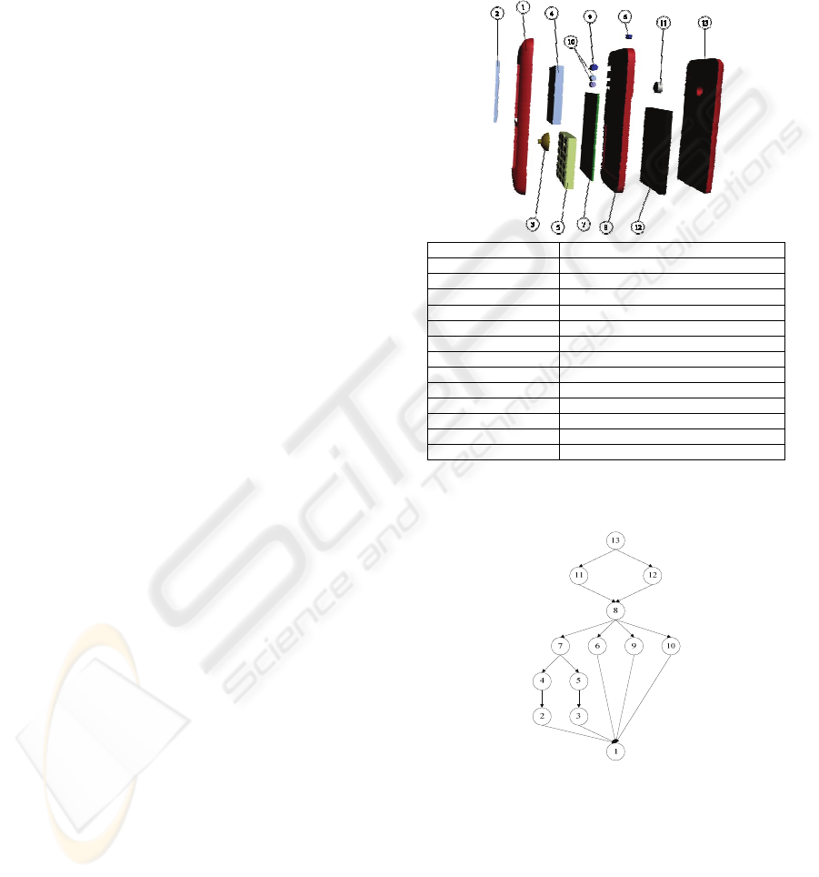
As shown in Figure 1, the example product A is

a mobile phone with 13 main components. The

APG of the product A is shown in Figure 2.

3.2 Assembly Precedence Matrix

(APM)

An APG is transformed into an assembly

precedence matrix (APM) for use in the PSO.

⎥

⎦

⎤

⎢

⎣

⎡

===

nnnn

njjj

bbb

ccc

###

12111

(2)

where c

and c

are components,

= 1 represents that component c

must be

assembled before component c

APM for the example product A =

000000000000013

100000000000012

100000000000011

111001000000010

111001000000009

111000000000008

111001000000007

111

001000000006

111001100000005

111001100000004

111001101000003

111001100100002

111111111111001

13121110090807060504030201

3.3 Plant Capability Table (PCT)

A plant capability table (PCT) is developed for use

in the plant selection and assignment. The general

form of a PCT is shown in Table 1. In the table, a

value of t

= 1 indicates that the component c

can be

A DECISION SUPPORT SYSTEM FOR MULTI-PLANT ASSEMBLY SEQUENCE PLANNING USING A PSO

APPROACH

125

assembled in the plant f

. The PCT of the product A

is shown in Table 2.

4 SOLUTION USING PARTICLE

SWARM OPTIMIZATION (PSO)

A PSO algorithm is presented for simultaneously

performing assembly sequence planning and plant

assignment. The PSO algorithm is an evolutionary

computation method introduced by Kennedy and

Eberhard (1995, 1997). In PSO, each particle

moves around in the multi-dimensional space with a

position and a velocity. The velocity and position

are constantly updated by the particle’s own

experience and the experience of the whole swarm.

Given a problem, a particle can be encoded to

represent a solution. Each solution, called a particle,

flies in the search space towards the optimal

position.

A particle is defined by its position and velocity.

The position of a particle i in the D-dimension

search space can be represented as X

=[x

, x

, …,

, …, x

]. The velocity of the particle i in the D-

dimension search space can be represented as

=[v

, v

, …, v

]. Each particle has its

own best position P

=[p

, p

, …, p

]

representing the particle’s personal best objective

(pbest) at time t. The global best particle is denoted

as p

and the best position of the entire swarm

(gbest) is denoted as P

=[p

, p

, …, p

] at

time t. To search for the optimal solution, each

particle adjusts its velocity according to the velocity

updating equation and position updating equation.

()

idgdidid

old

idi

new

xprcxprcvwv −⋅⋅+−⋅⋅+⋅=

2211

(3)

where d =1, …, D, i =1, …, E (number of particles),

new

: the new velocity of i in the current iteration t,

old

: the velocity of i in the previous iteration (t - 1),

and c

: constants called acceleration coefficients,

: the inertia weight,

and r

: two independent random numbers with a

uniform distribution [0, 1],

: the best position of each individual particle i,

: the best position of the entire swarm.

new

old

new

vxx +=

(4)

where

new

is the new position in the current

iteration t,

old

x is in the previous iteration (t - 1).

4.1 Encoding Scheme

In the developed encoding scheme, a particle

represents a feasible multi-plant assembly sequence.

A heuristic sequencing and assignment rule for

encoding and decoding is introduced as follows.

The position of particle i is represented by a

position matrix, denoted as X

ijk

, j = 1, …, (M+1), k =

1, …, N, where N is the number of components and

M is the number of plants. In the heuristic

sequencing rule, the values in the first row S of R

, …, R

represent the ranked order values of the

N components in an assembly sequence.

In each column, the values from row F

to row

represent the ranked assignment values for plant

assignment of a component. In the heuristic

assignment rule, the component C

is assigned to the

plant with the smallest value in the column of R

, …, R

ijk

⎥

⎦

⎤

⎢

⎣

⎡

MNMkMM

sNskss

RRRR

CCCC

222221

111211

)

where i = 1, …, E, where F

is a plant, j =1, …, M,

and C

is a component, k =1, …, N,

represents the ranked order value of a

component k,

represents the ranked assignment value for

component k assigned to plant j.

In the heuristic rule for assembly sequencing,

the values in [R

, R

, …, R

] are sorted in

an ascending order. The ranked order values

represent the ordered position of component C

the assembly sequence. For example, if the values

of row S are [4.5 1.1 3.2 7.6 5.3], then the ordered

positions of (C

, C

) are (third, first,

second, fifth, fourth). The assembly sequence is

determined as (C

, C

In the heuristic rule for plant assignment, in

each column of C

, the component C

is assigned to

the plant with the smallest ranked assignment value

in R

, for j = 1, …, M. For example, if there are

four plants, the values of column C

are [3.1 5.8

1.5 6.9]

, then the smallest value is 1.5 of plant F

Therefore, the component C

is assigned to plant F

4.2 Fitness Function

The cost functions include two major items. The

assembly operational costs are mainly related to

ICEIS 2009 - International Conference on Enterprise Information Systems

126

assembly sequencing, whereas the multi-plant costs

are primarily related to the plant assignment.

(1) Assembly operation cost (AOC): The assembly

operation cost is the basic operational cost for

performing an assembly operation.

(2) Assembly tool change cost (ATC): To perform

the assembly operation, proper tools are

required. If two tools are different, then an

assembly tool change cost is required.

(3) Assembly setup change cost (ASC): If two

consecutive setups are different, then an

assembly setup change cost is required.

(4) General transportation cost (GTC): Proper

transportation cost for moving and handling

between different plants needs to be defined.

The total cost function (TC) can be

formulated as follows (unit: dollars).

TC = AOC + ATC + ASC +GTC (6)

In the PSO evaluation, the objective is to

minimize the fitness function as follows.

Min Fitness = TC, (7)

Fitness: the fitness function value of a particle.

4.3 The PSO Algorithm for Multi-plant

Assembly Sequence Planning

The flowchart is shown in Figure 3.

Step 1. Setup parameters.

(1) Set iteration t = 0.

(2) T

Number

: the iteration (generation) number.

(3) P

Size

: the number of particles.

Step 2. Initialize a population of particles i = 1, …,

E,with random positions and velocities.

(1) A particle i is defined by a multi-dimensional

position matrix of (N)*(M+1).

(2) The position of particle i is defined by X

ijk

(3) The velocity of particle i is defined by V

ijk

Step 3. Evaluate the fitness function.

(1) t = t + 1.

(2) Fitness = TC.

Step 4. Update the velocity of each particle i.

(

)

()

idgdidid

old

idi

new

xprcxprcvwv −⋅⋅+−⋅⋅+⋅=

2211

new

v is the new velocity in the current iteration t,

old

v is the velocity in the previous iteration (t-1),

Step 5. Move the position of each particle i.

new

old

new

vxx +=

where

new

x is the new position in the iteration t,

old

x is the position in the iteration (t - 1).

Step 6. Check the feasibility of the solution and the

number of iteration t.

(1) The precedence is checked by APM.

(2) The plant capability is checked by PCT.

(3) If (t

> T

Number

), then go to Step 7, else go to

Step 2.

Step 7. Decode the best particle position and

interpret the solution.

5 IMPLEMENTATION AND TEST

RESULTS

In the presented decision support system, the models

were implemented and tested by developing

software on a personal computer with a 3.0 GHz

CPU and 1 GB memory. The example product A as

illustrated in Figure 1 is modelled and tested. The

product A is a mobile phone with 13 main

components. There are 4 available plants. The

APG of the product A is shown in Figure 2. The

APM of the product A is listed in the section 3 as

described earlier. The PCT of the product A is

shown in Table 2. The numerical values of the PSO

parameters are tested with an experiment using a

Taguchi’s orthogonal array to find the best

combination of parameters of T

Number

= 80, P

Size

20, w

= 0.9, and (c

) = (2, 2).

Figure 4 shows that the computation converges

after 32 generations with a cost of 258 (unit: dollars)

and a computer time of 0.0312 (unit: seconds). The

position matrix of the final solution is shown in

Table 3. As shown in Table 4, the position matrix

of the solution particle is decoded into assembly

sequence and plant assignment information. The

assembly sequence can be listed as C

-C

The plant assignment

information shows that the components C

-C

are assigned to plant F

. The components C

-C

are assigned to plant F

. The components

-C

are assigned to plant F

. Finally, the

component C

is assigned to plant F

to complete the

final product. As observed from the illustrative

example, it shows that the developed model and

algorithm present a feasible and efficient solution

method.

6 CONCLUSIONS

In this research, a decision support system with a

A DECISION SUPPORT SYSTEM FOR MULTI-PLANT ASSEMBLY SEQUENCE PLANNING USING A PSO

APPROACH

127

new multi-plant assembly planning model is

presented to perform two tasks, assembly sequence

planning and plant assignment. A PSO algorithm is

developed for simultaneously optimizing assembly

sequence planning and plant assignment. First, an

assembly precedence graph (APG) is built. The

assembly precedence matrix (APM) is modeled for

checking feasibility of the sequences. The plant

capability information is modeled in the plant

capability table (PCT). Next, a PSO algorithm is

presented to search for the solutions. A new PSO

encoding scheme is developed for assembly

component sequencing and plant assignment. A

particle is represented as a position matrix defined

by the number of components and the number of

plants. The fitness function is formulated by

integrating assembly operation cost, assembly tool

change cost, assembly setup change cost, and

general transportation cost. The test results show

that the PSO method converges fast to reach a

minimized cost objective. It can be generally

concluded that the developed models and the PSO

algorithm are feasible and efficient for solving

multi-plant assembly sequence planning. Future

research should be concerned with detailed analysis

of the parameters and investigation of the problem

complexity to reduce computational time.

REFERENCES

Abdullah, T. A., Popplewell, K., and Page, C. J. (2003). A

review of the support tools for the process of assembly

method selection and assembly planning, International

Journal of Production Research, 41(11), 2391–2410.

Banks, A., Vincent, J., and Anyakoha, C. (2008). A

review of particle swarm optimization. Part II:

hybridization, combinatorial, multicriteria and

constrained optimization, and indicative applications,

Natural Computing, 7, 109-124.

Dong, T., Tong, R., and Zhang, L. (2007). A knowledge-

based approach to assembly sequence planning,

International Journal of Advanced Manufacturing

Technology, 32, 1232-1244.

Kennedy, J., and Eberhart, R. C. (1995). Particle swarm

optimization, Proceedings of the IEEE International

Conference on Neural Networks, Piscataway, NJ,

1942-1948.

Kennedy, J., and Eberhart, R. C. (1997). A discrete binary

version of the particle swarm algorithm, Proceedings of

the International Conference on Systems, Man and

Cybernetics, Piscataway, NJ, 4104-4109.

Lai, H.-Y., and Huang, C.-T. (2004). A systematic

approach for automatic assembly sequence plan

generation, International Journal of Advanced

Manufacturing Technology, 24, 752-763.

Lin, A. C., and Chang, T. C. (1993). An integrated

approach to automated assembly planning for three-

dimensional mechanical products, International Journal

of Production Research, 31(5), 1201-1227.

Su, Q. (2007). Computer aided geometric feasible

assembly sequence planning and optimizing,

International Journal of Advanced Manufacturing

Technology, 33, 48-57.

Component Name

1 Top case

2 Screen cover

3 Main button set

4 LCD panel

5 Keyboard

6 Top button

7 Printed circuit board

8 Frame

9 Right button (Camera)

10 Right button(Sound)

11 Camera lens set

12 Battery

13 Bottom case

Figure 1: The example product A is a mobile phone with

13 main components.

Figure 2: The APG of the example product A.

ICEIS 2009 - International Conference on Enterprise Information Systems

128

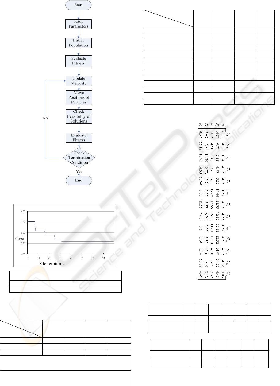
Figure 3: The flowchart of the PSO algorithm.

Cost (dollars) 258

Iterations (Generations) 32

Computer time (seconds) 0.0312

Figure 4: The test result of the PSO for product A.

Table 1: General format of PCT.

Plant f

Component p

1 2 … m

1 t

2 t

n t

= 1 indicates that p

can be assembled in f

= 0 indicates that p

cannot be assembled in f

Table 2: The PCT of the product A.

Plant

Component p

1 0 0 1 1

2 1 1 0 0

3 1 1 0 0

4 1 1 0 0

5 1 1 0 0

6 0 0 1 1

7 0 0 1 0

8 0 0 1 0

9 0 0 1 1

10 0 0 1 1

11 0 1 0 0

12 0 1 0 0

13 1 1 1 1

Table 3: The solution position matrix for product A.

Table 4: The solution of the multi-plant assembly

sequence for product A.

Assembly

sequence

1 2 3 4 5 6 7

Component 13 12 11 8 6 9 10

Assigned

plant

Assembly

sequence

8 9 10 11 12 13

Component 7 4 2 5 3 1

Assigned plant F

A DECISION SUPPORT SYSTEM FOR MULTI-PLANT ASSEMBLY SEQUENCE PLANNING USING A PSO

APPROACH

129