TEXTURED IMAGE SEGMENTATION BASED ON LOCAL
SPECTRAL HISTOGRAM AND ACTIVE CONTOUR
Xianghua Xie
Department of Computer Science, University of Wales Swansea, Swansea, U.K.
Keywords:
Active contour, Local spectral histogram, Level set method, Texture segmentation, Wasserstein distance.
Abstract:
In this paper, we propose a novel level set based active contour model to segment textured images. The pro-
posed methods is based on the assumption that local histograms of filtering responses between foreground and
background regions are statistically separable. In order to be able to handle texture non-uniformities, which
often occur in real world images, we use rotation invariant filtering features and local spectral histograms as
image feature to drive the snake segmentation. Automatic histogram bin size selection is carried out so that
its underlying distribution can be best represented. Experimental results on both synthetic and real data show
promising results and significant improvements compared to direct modeling of filtering responses.
1 INTRODUCTION
Active contours have been increasingly used in ana-
lyzing textured images, e.g. (Sandberg et al., 2002;
Ni et al., 2007; Houhou and Thiran, 2008; Savelonas
et al., 2008). Despite recent advances in edge based
approaches, e.g. (Paragios et al., 2004; Xie and
Mirmehdi, 2008), region based approaches have some
obvious advantages when analyzing heavily texture
images in that edge based boundary description can
easily be compromised by texture patterns. Region
based approach deforms initial contours towards the
region/object boundaries of interest by minimizing an
energy function, whose minimum ideally collocates
with those boundaries. Thus, it is vitally important
to use robust features and appropriate region indica-
tion/separation functional.
Various features have been investigated in the con-
tour segmentation framework, such as co-occurrence
matrices (Pujol and Radeva, 2004), structure ten-
sor (Rousson et al., 2004), and local binary patterns
(Savelonas et al., 2008). However, filtering responses
are among the most popular approaches, e.g. (Para-
gios and Deriche, 2002; Sandberg et al., 2002; Au-
jol et al., 2003; He et al., 2004; Sagiv et al., 2006).
In (Sandberg et al., 2002) the authors decompose the
image using Gabor filters. The collected filtering re-
sponses at each pixel are used to measure the differ-
ence between pixels in a piecewise constant model.
However, it largely ignores the spatial distribution
among local filtering coefficients and this direct com-
parison of filter responses is error prone since the re-
sponses can be misaligned due to the anisotropic na-
ture of most of the filters. Wavelet packet transform
is used in (Aujol et al., 2003) and the energy distribu-
tions in sub-bands are used to characterize textures.
One of the main difficulties in dealing with filtering
responses is their large dimensionality. It is also chal-
lenging to handle textural variations within regions of
interest due to, for example, rotation or view point
changes, since most of the filters are orientation sen-
sitive.
Once the features are derived, one also needs to
decide how to model their distributions so that cor-
rect features are included in describing the object of
interest. In other words, this modeling provides a re-
gion indication or separation functional to drive the
active contours. Modeling based on global distribu-
tion is a popular approach. For example, in (Paragios
and Deriche, 2002; He et al., 2004) Mixture of Gaus-
sians are used to model the image features. Another
powerful approach is based on the piecewise constant
assumption (Chan and Vese, 2001). It also has been
recently adopted in texture segmentation, e.g. (Sand-
berg et al., 2002; Sagiv et al., 2006; Ni et al., 2007).
However, how to cope with texture inhomogeneity is
a major challenge.
217
Xie X. (2009).
TEXTURED IMAGE SEGMENTATION BASED ON LOCAL SPECTRAL HISTOGRAM AND ACTIVE CONTOUR.
In Proceedings of the Fourth International Conference on Computer Vision Theory and Applications, pages 217-225
DOI: 10.5220/0001805502170225
Copyright
c
 SciTePress

2 PROPOSED APPROACH
In this paper, we propose a novel region based ac-
tive contour model, which is based on the assump-
tion that local histograms of filtering responses be-
tween object of interest and background regions are
statistically separable. Briefly, we first apply a bank
of filters to the image, from which we have a set of
filter responses at different scales and orientations.
These responses are then grouped and condensed so
that it can handle textural non-uniformity which may
occur in real world images. Reduced, invariant fea-
tures are thus obtained. This process also effectively
decreases the dimensionality of filter feature space,
which is beneficial for single image segmentation.
We then collect local distributions of these features
at each pixels, known as local spectral histograms.
These local histograms contains not only directly fil-
tering responses but also their spatial distributions in
their local neighborhoods. The optimal bin size for
these histograms are obtained by minimizing a mean
integrated square error based cost function. An en-
ergy minimization problem is thus formulated by fit-
ting two spectral histograms, one of which is used to
approximate the foreground region and the other for
the background. We will show that this approach is
effective to handle texture inhomogeneity, compared
to, for example, direct modeling of filtering responses
(Sandberg et al., 2002) or local intensity distributions
(Ni et al., 2007).
Next, Section 2.1 describes the filter bank and ro-
tation invariant feature selection. Local spectral his-
togram extraction is presented in Section 2.2 and au-
tomatic optimal histogram bin size computation is
given in Section 2.3. Finally, Section 2.4 introduces
the level set based snake model using these invariant
features for image segmentation.
2.1 Filters and Feature Selection
Texture provides important information for recogni-
tion and interpolation. Numerous techniques have
been reported in the literature to carry out texture
analysis. They can be generally categorized in four
ways: statistical approaches which measure the spa-
tial distribution of pixel values, structural approaches
that are based on analyzing texture primitives and the
spatial arrangement of these primitives, filter based
approaches which analyze local pixel dependencies
using a bank of filters, and model based approaches
which often use derived model parameters as texture
features. Filter bank based approaches have been pop-
ular since they can analyze textures in arbitrary orien-
tations and scales and have been strongly motivated
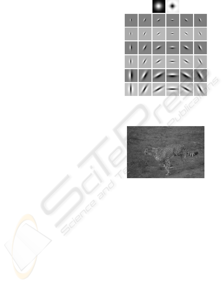
Figure 1: The filter bank consists 38 filters in total, which
include one Gaussian filter, one Laplacian of Gaussian fil-
ter, and 36 edge and bar filters across 6 orientations and 3
scales.
Figure 2: An example testing image.
by psychological studies of human vision system.
However, filter bank based methods often result
in high dimensional feature space which can be diffi-
cult to handle for certain applications. Unlike image
classification, in snake based image segmentation, we
may not have enough features extracted from a sin-
gle image to populate the high dimensional feature
space in order to accurately estimate the underlying
feature distributions. Moreover, there are usually sig-
nificant amount of redundant information among the
filtering responses. For example, a set of anisotropic
filters will get the same responses from isotropic im-
age regions. Fig. 1 shows a bank of filters which
has been used in (Varma and Zisserman, 2002) for
image classification. It contains two isotropic filters
and thirty six anisotropic filters. The two isotropic
filters are Gaussian and Laplacian of Gaussian both
with σ = 10. Those thrifty six anisotropic filters
come from two families, edges and bars, each of
which consists filters at three progressive scales, i.e.
(σ
x
,σ
y
) = {(1, 3), (2, 6),(4,12)}, and six uniformly
VISAPP 2009 - International Conference on Computer Vision Theory and Applications
218

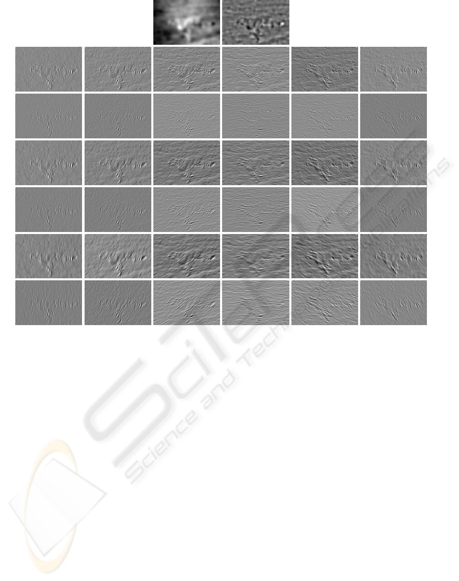
Figure 3: Filter responses.
spaced different orientations. This moderate size fil-
ter bank will produce a thirty eight dimensional fea-
ture space, which is considerably large for features
extracted from a single image to populate. Fig. 3
gives the filter responses of the example image shown
in Fig. 2. It is evidently clear that there are certain
correlations among these filter responses and not all
the channels are effectively revealing the image struc-
tures. Thus, it is natural to condense the feature space,
which is particularly desirable for our application.
It is also worth noting that object in the scene may
have inhomogeneous textures due to, for example,
perspective projection. This inhomogeneity will ex-
hibit nonuniform responses after applying directional
filters, e.g. animal stripe texture (see zebra exam-
ple in Fig. 7) and brick wall texture (see Fig. 8).
Rotation invariance is thus desirable in such circum-
stance. We follow (Varma and Zisserman, 2002) to
condense the filter responses by collecting only the
maximum filter response across all the six orienta-
tions, i.e. those thirty six directional filter responses
are reduced to six. Alternative methods, such as steer-
able filters (Jacob and Unser, 2004) can also be used.
Thus, this not only reduces the dimensionality of the
feature space but also simultaneously achieves rota-
tional invariancy.
Instead of applying convolution operators, the re-
cursive technique (Geusebroek et al., 2003) is used to
efficientlyfilter the images. Fig. 4 showsthe collected
maximum responses from those thirty eight filter co-
efficients. Note the isotropic filter responses are re-
main unchanged since they are inherently rotationally
invariant.
2.2 Local Spectral Histogram
The filtering responses can be directly used to drive
the active contours as in, for example, (Sandberg
et al., 2002). However, we can further incorpo-
rate local spatial dependency of filtering responses
by computing the marginal distributions of filter re-
sponses over a local window. Thus, it captures lo-
cal pixel dependency through filtering and global pat-
terns through histograms. Local spectral histogram
has been found useful, for example, texture classifi-
cation (Liu and Wang, 2003). The maximum filter
responses are largely local dominant features, such as
edges and bars (e.g. see 4). Their spatial distribu-
TEXTURED IMAGE SEGMENTATION BASED ON LOCAL SPECTRAL HISTOGRAM AND ACTIVE CONTOUR
219

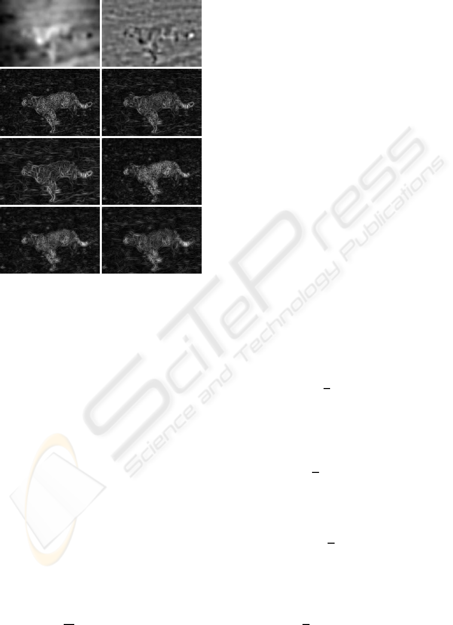
Figure 4: Maximum filter responses - The first row shows
the filter responses from the isotropic Gaussian and Lapla-
cian of Gaussian are kept the same. The rest six filter re-
sponses are collected from the 36 directional (isotropic)
filter responses. Each of them contains the maximum re-
sponses across 6 different orientations (i.e. the six rows of
the directional filter responses in Fig. 3 are collapsed into
six rotational invariant filter responses).
tion conveys important information regarding the na-
ture of the texture. Misaligning of filter responses due
to inhomogeneity of filter responses can be a serious
problem for direct approaches. Using local spectral
histogram further enhances our model in dealing with
texture inhomogeneity and helps to produce more co-
herent segmentation. Fig. 8 provides an example
where directly using filter response and without tak-
ing into texture inhomogeneity resulted in a very poor
segmentation, while as the proposed method correctly
segmented the foreground object from the texturally
nonuniform background.
Let W denote a local window and W
(α)
(x) a max-
imum filter response patch centered at x, where α =
1,2,...,8. Thus, for W
(α)
the histogram is defined as
(Liu and Wang, 2006):
P
(α)
W
(z
1
,z
2
) =
∑
x∈W
Z
z
2
z
1
δ(z− W
(α)
(x))dz, (1)
where z
1
and z
2
specify the range of the bin. The spec-
tral histogram is then defined as:
P
W
=
1
W

P
(1)
W
,P
(2)
W
,...,P
(8)
W
,

. (2)
Example spectral histograms extracted from the test-
ing image can be found in Fig. 6.
Very recently in (Ni et al., 2007), local image in-
tensity histogram was used in the Chan-Vese model
(Chan and Vese, 2001). However, this method may
have difficulties in dealing with highly textured im-
ages where intensity alone is not sufficient to describe
the texture. Intensity variation, for example, due to il-
lumination changes can also cause severe problems.
A comparative example is given in 9 where the best
result reported in (Ni et al., 2007) is still significantly
less accurate than the proposed approach.
2.3 Deducing Optimal Bin Size
Although histogram based methods have been rou-
tinely used in various image processing tasks, the im-
portance of automatically selecting appropriate his-
togram bin size has been largely ignored. However,
if a too small bin size is selected, the frequency value
at each bin will suffer from significant large fluctua-
tion due to the paucity of samples in each bin. On
the other hand, if the bin size is chosen too large, the
histogram will not be a good representation of the un-
derlying distribution. Thus, it is necessary to select
an optimal bin size. It also avoids the practical issues
associated with manual parameter tunning.
We follow the method in (Shimazaki and Shi-
nomoto, 2007) to estimate the optimal bin size. Let
us consider a histogram as a bar graph. Also, let ∆ de-
note the bin size. Theexpected frequencyfor s ∈ [0, ∆]
is:
θ =
1
∆
Z
∆
0
λ
s
ds, (3)
where λ
s
is the underlying true frequency which is not
known. The goodness of fit of the estimated
ˆ
λ
s
to λ
s
is
measured according to mean integrated squared error
(MISE):
MISE =
1
∆
Z
∆
0
hE(
ˆ
θ− λ
s
)
2
ids, (4)
where E denotes expectation and the empirical bar
height
ˆ
θ
i
≡ k
i
/∆ (k
i
is the frequency count for ith bin).
The associated cost function is then defined as:
O (∆) = MISE−
1
∆
Z
∆
0
h(λ
s
− hθi)
2
ids. (5)
The second term represents a mean squared fluctua-
tion. By assuming the number of events counted in
each bin obeys a Poisson distribution, the cost func-
tion can be written as:
O (∆) =
2
∆
hE
ˆ
θi − hE(
ˆ
θ− hE
ˆ
θi)
2
i. (6)
VISAPP 2009 - International Conference on Computer Vision Theory and Applications
220

−1.5 −1 −0.5 0 0.5 1 1.5 2 2.5
0
200
400
600
800
1000
1200
Coefficient
Frequency
0 0.1 0.2 0.3 0.4 0.5 0.6 0.7 0.8 0.9
−8.5
−8
−7.5
−7
−6.5
−6
−5.5
−5
x 10
7
Bin size
Cost
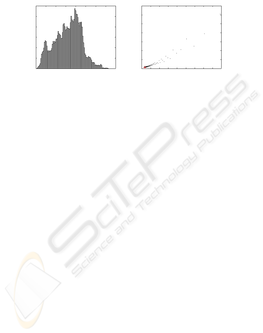
Figure 5: Optimal bin size selection - left: A typical spectral histogram for a single maximum response filter; right: The plot
shows the relationship between the MISE based cost function and bin size (the red cross indicates the optimal bin size with
the lowest MISE value).
The optimal bin size thus is obtained by minimizing
the above cost function, i.e.
ˆ
∆ = argmin
∆
O (∆). (7)
Thus, the testing image is first filtered through
the bank of isotropic and anisotropic filters and their
responses are condensed into eight channels. Local
spectral histograms at each pixel position are com-
puted and histograms from the same channel are put
together to produce a global histogram, i.e. mean lo-
cal spectral histogram. Then, this optimal bin size
selection is taken place for each of these eight mean
local spectral histograms. Finally, all the local spec-
tral histograms are finalized using the derived optimal
bin size values. Fig. 5 gives an example of optimal
bin size computation.
2.4 Active Contour based on
Wasserstein Distance
The snake based segmentation can be viewed as a
foreground-backgroundpartition problem (in the case
of bi-phase). The snake evolves in the image domain,
attempting to minimizing the feature similarity for
those inside and outside the contours. Meanwhile, it
tries to minimize the feature difference for those that
are belong to the same region. Thus, we can formulate
our snake based on the piece-wise constant assump-
tion (Chan and Vese, 2001; Ni et al., 2007). However,
since we are using invariant image features and local
spectral histograms, the proposed method can cope
with texture inhomogeneitymuch better than the orig-
inal piece-wise constant model (see Figs. 8 and 9 as
comparative examples).
Let Ω be the image domain, Λ
+
denote the re-
gions inside the snake (foreground)and Λ
−
those out-
side the snake (background). The snake segmentation
can be achieved by solving the following energy min-
imization problem:
inf
Λ
+
E (Λ
+
) =αL (Λ
+
)
+
Z
Λ
+
D (P(x),P
+
)dx (8)
+
Z
Λ
−
D (P(x),P
−
)dx,
where α is a constant, L denote length, D is the met-
ric which measures the difference between two his-
tograms, and P
+
and P
−
are the foreground and back-
ground mean local spectral histograms to be deter-
mined. The first term is the length minimization term
which regularize the contour. The next two terms are
data fitting terms, which carry out the binary segmen-
tation.
Among many other candidates, such as χ
2
dis-
tance and normalized cross correlation, The Wasser-
stein distance (also known as the earth mover’s dis-
tance) (Rubner et al., 1998) is used to compute the
distance between two normalized spectral histograms.
since it is a true metric (unlike χ
2
distance) and has
been found very useful in various applications, e.g.
image retrieval (Rubner et al., 1998). Let H
a
(y) and
H
b
(y) be two normalized spectral histograms. The
Wasserstein distance between these two histograms is
defined as:
D (P
a
,P
b
) =
Z
T
|F
a
(y) − F
b
(y)|dy, (9)
where T denoted the range of the histogram bins, and
F
a
and F
b
are cumulative distributions of P
a
and P
b
,
respectively.
The level set method is implemented to solve
this energy minimization problem so that topological
changes, such as merging and splitting, can be effec-
tively handled. Let φ denote the level set function.
The foreground is identified as Λ
+
= { x ∈ Ω : φ(x) >
TEXTURED IMAGE SEGMENTATION BASED ON LOCAL SPECTRAL HISTOGRAM AND ACTIVE CONTOUR
221

0 100 200 300 400 500 600 700 800 900 1000
0
0.02
0.04
0.06
0.08
Histogram bin
Frequency
outside
inside
0 100 200 300 400 500 600 700 800 900 1000
0
0.02
0.04
0.06
0.08
0.1
Histogram bin
Frequency
outside
inside
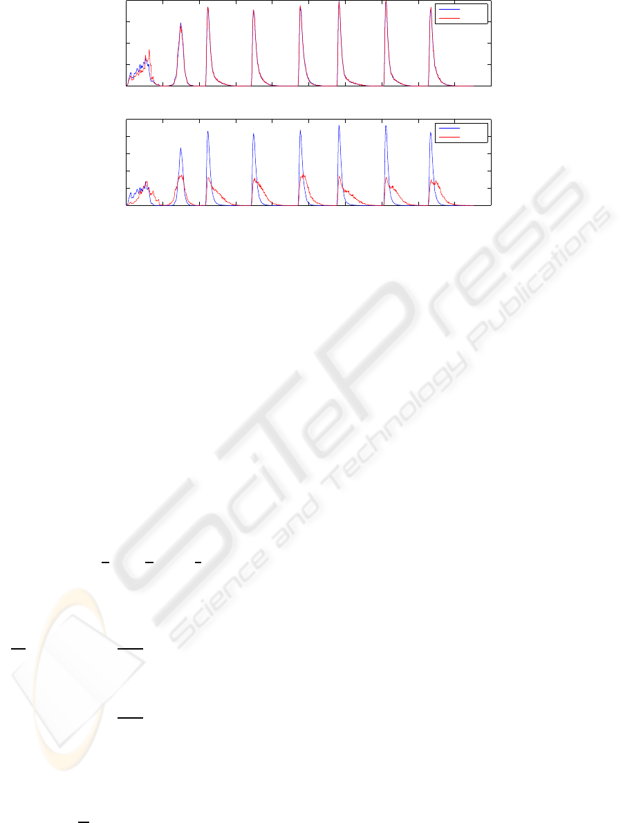
Figure 6: The average local spectral histogram inside and outside the snake - top: These two histograms are largely over-
lapping each other; bottom: It clearly shows the difference between the histograms when the snake converged to the object
boundaries.
0}, which can be computed using the Heaviside func-
tion, i.e.
R
Ω
H (φ)dx where H is the Heaviside func-
tion. The level set formulation can be expressed as:
inf
Λ
+
E (Λ
+
) =α
Z
Ω
|∇H (φ)|dx
+
Z
Ω
D (P(x),P
+
)H (φ)dx (10)
+
Z
Ω
D (P(x),P
−
)(1− H )(φ)dx
The regularized Heaviside function proposed in
(Chan and Vese, 2001) is used to allow larger support
in the vicinity of the zero level set so that the contours
can be initialized anywhere across the image (e.g. see
Fig. 7):
H
ε
(z) =
1
2

1+
2
π
arctan(
z
ε
)

. (11)
Thus, minimizing E with respect to φ gives us the
following partial differential equation:
∂φ
∂t
= δ
ε
(φ)
h
α∇·

∇φ
|∇φ|

− (D (P(x),P
+
) − D (P(x),P
−
))
i
= δ
ε
(φ)
h
α∇·

∇φ
|∇φ|

−
Z
T
|F
x
(y) − F
+
(y)|dy
+
Z
T
|F
x
(y) − F
−
(y)|dy
i
, (12)
where δ
ε
(x) =
d
dx
H
ε
(x), F
+
and F
−
are the spectral
cumulative histogram inside and outside the contours,
respectively. The minimization process thus moves
the contours towards object boundaries through com-
peting pixels by measuring the similarity of local cu-
mulativespectral histogram with those inside and out-
side current foreground.
Fig. 6 shows an example of spectral histogram
changes between the initial stage and the stabilized
result. The corresponding segmentation result can be
found in the first row of Fig. 7.
3 RESULTS
The proposed method have been tested on both syn-
thetic and real world images. Fig. 7 shows some
typical examples results obtained using the proposed
method. The first row shows the result of the run-
ning example given earlier. Good segmentation was
achieved despite the large variations in the body re-
gion. In the second example, reasonable result was
obtained, missing some very fine and thin structures.
In the third example, there are clearly texture orienta-
tion variations. In the last two rows, the initial snakes
were placed outside the objects of interest but still
managed to localize them. Particularly, in the last ex-
ample, there are significant texture variations both in
foreground and background regions, which made it
very difficult to segment.
In Figs. 8 and 9, we mainly compare our work
with two extensions of the piece-wise constant model,
which is also our fundamental model. Fig. 8 demon-
strates when dealing with inhomogeneous textures,
the proposed method performs significantly better
than that directly using filter responses (Sandberg
et al., 2002). The proposed method also showed im-
provements against a very recent method based on lo-
VISAPP 2009 - International Conference on Computer Vision Theory and Applications
222

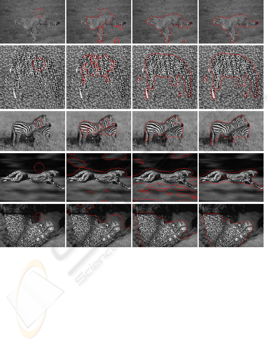
Figure 7: Examples results of the proposed method - from left: initial snake, intermediate stages, and stabilized results.
cal histograms (Ni et al., 2007). It illustrates the ef-
fectiveness of using invariant filtering technique. Fig.
9 also gives example results obtained from geodesic
snake and generalized GVF snake (Xu and Prince,
1998). It is expected that these edge based techniques
are not appropriate when dealing with highly textured
images.
The proposed method requires very little parame-
ter tunning. All the images given in this paper are us-
ing a fixed set of parameters. The parameters used to
generate the filter bank are given in Section 2.1. The
local window used to collect the spectral histogram
is empirically fixed as 19. For a too small window
size, the local spectral histogram may have difficulties
in reflecting underlying distribution and can result in
isolated regions. For a too large window, the segmen-
tation can be less accurate around object boundaries.
We found that a window size of 19 is a good trade-
off, however, we attempt to automatically select the
window size as part of our future work. The parame-
ter α controls the smoothness of the contour and very
rarely needs adjustment. As for computational com-
plexity, the proposed method is very similar to (Sand-
berg et al., 2002).
4 CONCLUSIONS
In this paper, we introduced a novel region based
snake method which is based on the assumption that
foreground and background local filtering response
distributions are statistically separable. Maximum re-
TEXTURED IMAGE SEGMENTATION BASED ON LOCAL SPECTRAL HISTOGRAM AND ACTIVE CONTOUR
223

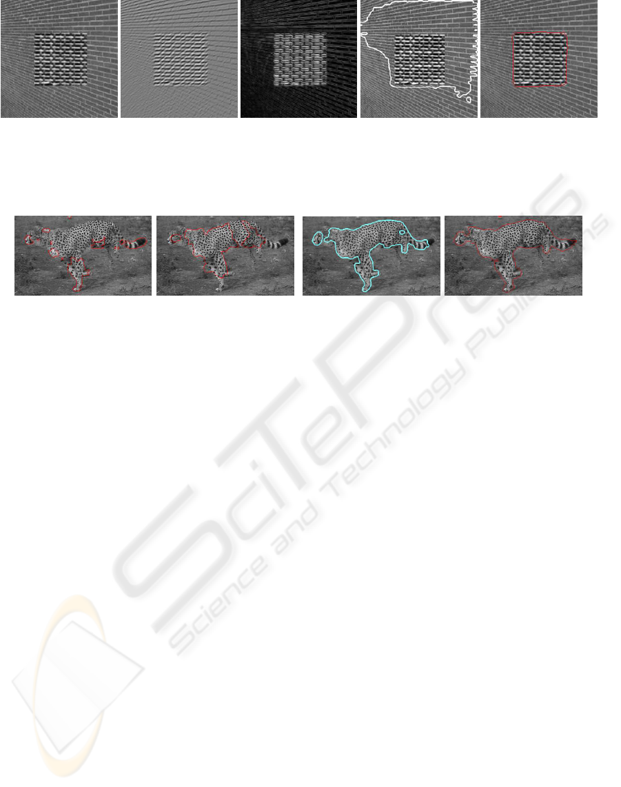
Figure 8: From left: a synthetic texture collage which contains an inhomogeneous background due to orientation and scale
changes; a filter response to a particular orientation; the maximum response derived across different orientations which
highlights edge features in various directions, including vertical; segmentation result obtained using the Chan-Vese model
based on Gabor features (Sandberg et al., 2002) (result reported in(Sagiv et al., 2006)); segmentation result obtained using the
proposed method.
Figure 9: Comparative analysis - first two images: results obtained using edges based methods, namely geodesic snake and
generalized GVF snake (Xu and Prince, 1998); third image: best result on the testing image reported in (Ni et al., 2007) using
a region based approach; last image: result obtained using the proposed method.
sponses filters were used to achieve rotational invari-
ancy and their local spectral histograms were used as
image features to drive the snake. The experimental
studies showed some very promising results. As part
of our future work, we will further investigate optimal
filter selection and automatic local spectral histogram
window selection.
ACKNOWLEDGEMENTS
The recursive filtering is based on the library provided
by (Geusebroek et al., 2003).
REFERENCES
Aujol, J., Aubert, G., and Blanc-F´eraud, L. (2003).
Wavelet-based level set evolution for classification of
textured images. IEEE T-IP, 12(12):1634–1641.
Chan, T. and Vese, L. (2001). Active contours without
edges. IEEE T-IP, 10(2):266–277.
Geusebroek, J., Smeulders, A., and van de Weijer, J.
(2003). Fast anisotropic gauss filtering. IEEE T-IP,
12(8):938–943.
He, Y., Luo, Y., and Hu, D. (2004). Unsupervised texture
segmentation via applying geodesic active regions to
Gaborian feature space. IEEE Trans. Eng. Comput.
Technol., pages 272–275.
Houhou, N. and Thiran, J. (2008). Fast texture segmentation
model based on the shape operator and active contour.
In IEEE CVPR, pages 1–8.
Jacob, M. and Unser, M. (2004). Design of steerable filters
for feature detection using Canny-like criteria. IEEE
T-PAMI, 26(8):1007–1019.
Liu, X. and Wang, D. (2003). Texture classification using
spectral histograms. IEEE T-IP, 12(6):661–670.
Liu, X. and Wang, D. (2006). Image and texture segmen-
tation using local spectral histograms. IEEE T-IP,
15(10):3066–3077.
Ni, K., Bresson, X., Chan, T., and Esedoglu, S. (2007). Lo-
cal histogram based segmentation using the Wasser-
stein distance. In Scale Space and Variational Meth-
ods in Computer Vision, pages 697–708.
Paragios, N. and Deriche, R. (2002). Geodesic active re-
gions and level set methods for supervised texture seg-
mentation. IJCV, 46(3):223–247.
Paragios, N., Mellina-Gottardo, O., and Ramesh, V. (2004).
Gradient vector flow geometric active contours. IEEE
T-PAMI, 26(3):402–407.
Pujol, O. and Radeva, P. (2004). Texture segmentation by
statistical deformable models. International Journal
of Image and Graphics, 4(3):433–452.
Rousson, M., Brox, T., and Deriche, R. (2004). Active un-
supervised texture segmentation on a diffusion based
feature space. In IEEE CVPR, pages 1–8.
Rubner, Y., Tomasi, C., and Guibas, L. (1998). A metric for
distributions with applications to image databases. In
IEEE CVPR, pages 59–66.
Sagiv, C., Sochen, N., and Zeevi, I. (2006). Integrated ac-
tive contours for texture segmentation. IEEE T-IP,
15(6):1633–1645.
Sandberg, B., Chan, T., and Vese, L. (2002). A level-set and
gabor-based active contour algorithm for segmenting
VISAPP 2009 - International Conference on Computer Vision Theory and Applications
224

textured images. Technical Report 39, Math. Depart-
ment UCLA, Los Angeles, USA.
Savelonas, M., Iakovidis, D., and Maroulis, D. (2008).
LBP-guided active contours. Pattern Recognition Let-
ters, 29(9):1404–1415.
Shimazaki, H. and Shinomoto, S. (2007). A method for se-
lecting the bin size of a time histogram. Neural Com-
putation, 19(6):1503–1527.
Varma, M. and Zisserman, A. (2002). Classifying images of
materials: Achieving viewpoint and illuminationinde-
pendence. In ECCV, pages 255–271.
Xie, X. and Mirmehdi, M. (2008). MAC: Magnetostatic
active contour model. IEEE T-PAMI, 30(4):632–646.
Xu, C. and Prince, J. (1998). Snakes, shapes, & gradient
vector flow. IEEE T-IP, 7(3):359–369.
TEXTURED IMAGE SEGMENTATION BASED ON LOCAL SPECTRAL HISTOGRAM AND ACTIVE CONTOUR
225