FAST MULTI-CLASS IMAGE ANNOTATION WITH RANDOM

SUBWINDOWS AND MULTIPLE OUTPUT RANDOMIZED TREES

Marie Dumont

, Rapha¨el Mar´ee

, Louis Wehenkel

1,2

and Pierre Geurts

1,2

Systems and Modeling - Department of Electrical Engineering and Computer Science

University of Li`ege, Sart-Tilman B28, B-4000 Li`ege, Belgium

Bioinformatics and Modeling - GIGA-R, University of Li`ege, Sart-Tilman B28, B-4000 Li`ege, Belgium

Keywords:

Image annotation, Machine learning, Decision trees, Extremely randomized trees, Structured outputs.

Abstract:

This paper addresses image annotation, i.e. labelling pixels of an image with a class among a ﬁnite set of

predeﬁned classes. We propose a new method which extracts a sample of subwindows from a set of annotated

images in order to train a subwindow annotation model by using the extremely randomized trees ensemble

method appropriately extended to handle high-dimensional output spaces. The annotation of a pixel of an

unseen image is done by aggregating the annotations of its subwindows containing this pixel. The proposed

method is compared to a more basic approach predicting the class of a pixel from a single window centered on

that pixel and to other state-of-the-art image annotation methods. In terms of accuracy, the proposed method

signiﬁcantly outperforms the basic method and shows good performances with respect to the state-of-the-art,

while being more generic, conceptually simpler, and of higher computational efﬁciency than these latter.

1 INTRODUCTION

In this paper, we propose a new supervised learn-

ing approach for fast multi-class image annotation.

Given a training set of images with pixel-wise la-

belling (i.e. every pixel is labelled with one class

among a ﬁnite set of predeﬁned classes), the goal is

to build a model to predict accurately the class of

every pixel of any new, unseen image. We distin-

guish this problem from image classiﬁcation (where

the goal is to assign classes to entire images), image

segmentation (where the goal is to partition images

into coherent regions without semantic labelling), ob-

ject detection (where the goal is to determine if an

object of a certain type is present in an image), and

image retrieval (where the goal is to retrieve images

similar to a set of given images). In some sense,

image annotation could be considered as the joint

detection, recognition, and segmentation of (multi-

ple) objects in one image. Image annotation is also

named image labelling in (He et al., 2004), simulta-

neous object recognition and segmentation in (Shot-

ton et al., 2006), background/foreground separation

or ﬁgure/ground segregation (when only two classes

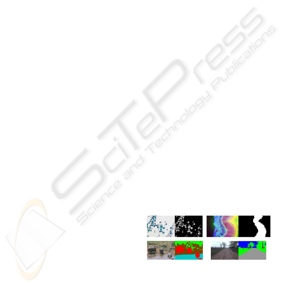
are deﬁned) in (Yu and Shi, 2003). Examples of im-

ages and their annotation are given in Figure 1. Since

manual annotation is labor intensive and some ap-

plications require the annotation of thousands of im-

ages, there is a strong need for automatic annotation

tools. Moreover, possible applications of such tech-

niques are numerous, eg. in aerial photographyanaly-

sis or in biomedical problems where high-throughput

microscopy systems can generate thousands of im-

ages daily that represent verydifferent phenotypes un-

der various experimental conditions. In this context,

generic methods that can automatically learn to adapt

to problem speciﬁcities are strongly needed.

Figure 1: Examples of images (left) with their manual an-

notation (right). Each color on the right images represents a

different class.

Several methods have been proposed in the lit-

erature to automatically annotate images. Some of

them are ad-hoc methods developed for speciﬁc im-

age families while others seek to be more generic.

196

Dumont M., Marée R., Wehenkel L. and Geurts P. (2009).

FAST MULTI-CLASS IMAGE ANNOTATION WITH RANDOM SUBWINDOWS AND MULTIPLE OUTPUT RANDOMIZED TREES.

In Proceedings of the Fourth International Conference on Computer Vision Theory and Applications, pages 196-203

DOI: 10.5220/0001800001960203

 SciTePress

In (Cour and Shi, 2007) and (Borenstein and Malik,

2006), a bottom-up approach is used to segment horse

images into coherent regions and a top-down method

groups the segments into larger regions. The method

of (Meurie et al., 2003) was applied to cell images

and consists in simplifying the images by ﬁltering, us-

ing a SVM pixel classiﬁer, realizing a marker extrac-

tion and ﬁnally, applying color watershed segmenta-

tion. In (Bertelli et al., 2007), a method is proposed to

separate foreground and background of retina images,

based on the minimization of a cost function express-

ing the dissimilarity between the image to annotate

and a reference image. Several authors (Shotton et al.,

2006; Shotton et al., 2007; He et al., 2004; Verbeek

and Triggs, 2007) have proposed to use conditional

random ﬁeld models for image annotation. These ap-

proaches differ in the features that are exploited in

the model (which are based on texture, shape, color,

layout, location...), the incorporation of local and/or

global information, and in the way the model param-

eters are learned.

Our starting point in this paper is the image clas-

siﬁcation method of Mar´ee et al. (Mar´ee et al., 2003;

Mar´ee et al., 2005) based on the extraction of ran-

dom subwindows, their description by raw pixel val-

ues, and their classiﬁcation by extremely randomized

trees (Geurts et al., 2006a). Randomization of patch

extraction was ﬁrst proposed in (Mar´ee et al., 2003)

for image classiﬁcation and subsequently in (Mar´ee

et al., 2005; Nowak et al., 2006). To the best of

our knowledge it was never considered for multi-class

pixelwise labelling. Different variants of randomized

trees were used in the recent years by an increas-

ing number of computer vision researchers, respec-

tively for content-based image retrieval (Mar´ee et al.,

2007; Philbin et al., 2007), keypoint tracking (Lepetit

and Fua, 2006) (inspired by (Amit and Geman, 1997)

for handwritten digit recognition), object categoriza-

tion (Bosch et al., 2007; Moosmann et al., 2006), vi-

sual identiﬁcation (Nowak and Jurie, 2007), bilayer

video segmentation (Yin et al., 2007), robot naviga-

tion (Jodogne et al., 2006; Ernst et al., 2006), image

reconstruction (Geurts et al., 2006b). Very recently

(Shotton et al., 2008), ensembles of randomized trees

were used to build bags of semantic textons for image

annotation. Another decision tree model, the Proba-

bilistic Boosting-Tree, was used in the context of the

detection of object boundaries (Dollar et al., 2006) to

classify as edge or non-edge the central pixel of image

patches described by roughly 50000 features.

The paper is structured as follows. We ﬁrst de-

scribe a basic pixel annotation method and then our

proposed method in Section 2. The ﬁrst one is

an adaptation of Mar´ee et al’s image classiﬁcation

method (Mar´ee et al., 2005) to classify each pixel

from a subwindow centered on it. The proposed ap-

proach exploits a multiple output extension of deci-

sion trees to simultaneously annotate all pixel labels

of a subwindow. In Section 3, these methods are con-

fronted on a diverse set of problems taken from the

literature to assess their generality and compare their

performances. We also analyse these two methods in

terms of computing times and parameter sensitivity.

Finally, we conclude and provide future work direc-

tions in Section 4.

2 METHODS

In Section 2.1, we brieﬂy remind the basic princi-

ples behind the image classiﬁcation method of (Mar´ee

et al., 2005). Section 2.2 describes our two extensions

for dealing with the image annotation problem.

2.1 Image Classiﬁcation

The goal of image classiﬁcation is to build, from a

learning sample of images, each labelled with a class

among a set of predeﬁned classes, a classiﬁer able to

predict as well as possible the class of unseen images.

To this end, the method described in (Mar´ee et al.,

2003; Mar´ee et al., 2005) ﬁrst randomly extracts a

large set of image subwindows and describes them by

feature vectors composed of raw pixel values. Each

subwindow is labelled with the class of its parent im-

age. Then, a supervised learning method is used to

build a subwindow classiﬁcation model from these

subwindows. At the prediction stage, subwindows are

extracted from the unseen image and classiﬁed by the

subwindow classiﬁer. These predictions are then ag-

gregated to get a single class prediction for the whole

image.

In principle, any supervised classiﬁcation method

can be used to grow the subwindow classiﬁers. Mar´ee

et al. exploited a particular decision tree ensemble

method, called extremely randomized trees or Extra-

Trees (Geurts et al., 2006a). This method grows an

ensemble of M (typically M ∈ [10;100]) unpruned

trees, each one being created in a top-down fash-

ion. With respect to other tree-based ensemble meth-

ods such as Tree Bagging or Random Forests, Extra-

Trees select cut-points at random and use the whole

learning sample rather than a bootstrap replica. Their

node splitting algorithm depends on two parameters,

namely the size K of the random subset of attributes

considered at each split, and the minimal (sub)sample

size to split a node, n

min

. In our experiments in Sec-

tion 3, we will use the default value recommended in

FAST MULTI-CLASS IMAGE ANNOTATION WITH RANDOM SUBWINDOWS AND MULTIPLE OUTPUT

RANDOMIZED TREES

197

(Geurts et al., 2006a), i.e. K equal to the square root

of the total number of attributes and n

min

= 2 (corre-

sponding to fully developed trees). In Section 3.5, we

will discuss the inﬂuence of K on accuracy and com-

puting times.

2.2 Image Annotation

We address the problem of image annotation as fol-

lows: given a sample LS of images with every pixel

labelled with one class among a ﬁnite set of prede-

ﬁned classes, build a classiﬁer able to predict as accu-

rately as possible the class of every pixel of an unseen

image.

2.2.1 Subwindow Classiﬁcation Model (or SCM)

A ﬁrst obvious, but novel,extension of the image clas-

siﬁcation approach (Mar´ee et al., 2005) for dealing

with pixelwise labeling is to associate to each subwin-

dow the class of its central pixel and then to label the

pixels of an image with this classiﬁer. The different

steps of this approach are detailed below.

Learning Sample Generation. The learning sam-

ple of subwindows that will be used to create the sub-

window centralpixel classiﬁer is created by extracting

subwindows of ﬁxed size w×h at random positions in

training images. Each subwindow is then labeled by

the class of the central pixel in its parent image. Each

subwindow is described by the HSB values of its raw

pixels, yielding a vector of w ×h ×3 numerical at-

tributes.

Learning. From the learning sample created at the

previous step, a model is built using ensembles of

extremely randomized trees (following (Mar´ee et al.,

2005)). Each test associated to an internal node of

a tree simply compares a pixel HSB component to a

numerical threshold (T = [a < a

]). The search of the

best internal test among K random tests requires to de-

ﬁne a score measure. Different scores measures have

been proposed in the decision tree literature. In this

paper, we have chosen the Gini splitting rule of CART

(Breiman et al., 1984) (also used in Random Forests)

. Formally, this score measure is deﬁned as follows:

score(S,T) = G

(S) −G

C|T

(S), (1)

with

(S) =

∑

i=1

.(1−

), (2)

We did some comparison with a log entropy based

score that does not show any signiﬁcant difference. We

choose Gini entropy because it is faster to compute.

C|T

∑

j=1

∑

i=1

.(1−

. j

), (3)

where S is the subsample of size n

associated to

the node to split, m is the number of pixel classes,

(i = 1,...,m) is the number of subwindows in S

whose central pixel is of class i, n

(resp. n

) is the

total number of subwindows of S whose central pixel

is of class i and which satisfy (resp. do not satisfy)

the test T, while n

(resp. n

) is the number of sub-

windows of S which satisfy (resp. do not satisfy) T.

The vector of probabilities which is attributed to

each terminal node (or leaf) is computed by using the

subset S of LS reaching this node: the i-th element (i=

1,...,m) is the proportion of subwindows of S whose

central pixel is in the ith class.

Prediction Step. For each pixel a subwindow cen-

tered on it is extractedfrom thetest image and its class

is predicted using the Extra-Trees, by averaging the

class-probability vectors returned by the trees of the

ensemble and selecting the most probable class. Note

that when we extract the subwindow centered on a

pixel which is close to the borders of the image, we

simply consider that the part of the subwindow that is

out of the image is composed of black pixels.

Computational Complexity. The number of oper-

ations to build M trees from a learning sample of N

subwindows is O (M

√

whNlog

N). The classiﬁcation

of a pixelwith an ensemble of M balancedtrees grown

from a sample of N subwindows requires on the av-

erage O (Mlog

N) tests. The number of subwindows

to extract is equal to the number of image pixels. The

annotation is thus linear in the size of the image.

2.2.2 Subwindow Classiﬁcation Model with

Multiple Outputs (or SCMMO)

We now describe a second approach whose main dif-

ference with the previous one is that the subwindows

classiﬁer is extended so as to predict the class of all

subwindow pixels.

Learning Sample Generation. Random subwin-

dows of size w×h are extracted from training images

as in the previous method. The difference is that the

full annotation is associated to each subwindow.

Learning. Our idea here is to build a classiﬁer able

to predict at once a class for each pixel of a sub-

window (instead of only the central pixel). Several

extensions of decision trees have been proposed to

handle multiple outputs (eg. (Geurts et al., 2006b)).

These methods differ from the standard tree-growing

VISAPP 2009 - International Conference on Computer Vision Theory and Applications

198

method in the score measure used to select splits and

in the way predictions are computed at tree leaves.

The score measure that we propose here is the av-

erage of the Gini entropy based score for each output

pixel. More precisely, we have:

score(S,T) =

w.h

w∗h

∑

k=1

score

(S,T) (4)

score

(S,T) = G

(S) −G

C|T

(S) (5)

(S) =

∑

i=1

i.k

...

(1−

i.k

...

) (6)

C|T

∑

j=1

∑

i=1

ijk

...

(1−

ijk

. j.

), (7)

where the parameters have the same meaning as in

the previous section with the addition of the index k ∈

1,..., wh that references the subwindow pixels.

Once the tree is built, class probability estimates

at each subwindow position could then be obtained at

each leaf simply by computing class frequencies over

all subwindows that reach the leaf. However, the size

of such a probability vector is equal to the number of

pixels times the number of classes and thus the stor-

age of these vectors at each leaf node could require

a lot of memory space. To reduce this requirement,

in our implementation, we have decided to keep track

only of the majority class of each pixel together with

its conﬁdence as measured by its frequency. This sim-

pliﬁcation leads to memory requirements independent

of the number of classes

Prediction. The annotation process again consists

in extracting subwindows and in testing each one of

them with all the trees. To get a prediction for each

pixel, these subwindows need at least to cover the

whole image. However, we observed that the more

subwindows are extracted, the better the predictions.

Thus, in our experiment, we extracted all possible,

overlapping, subwindows.

By testing each subwindow with all the trees, a

set of tuples (class number,rate of conﬁdence) is as-

signed to each pixel of the initial image. From this set

of predictions, a vector of size m (number of different

classes) is computed for each pixel: its i-th element

(i = 1,...,m) is the sum of the conﬁdence numbers

which are associated to the i-th class among all pre-

dictions. The predicted class for the considered pixel

is the one that receives the highest overall conﬁdence.

We run several experiments keeping the full class prob-

ability vectors at tree leaves but no signiﬁcant difference

was observed.

Table 1: Main properties of the four datasets.

DB # Im. Im. size Protocol # Subwin.

per image

Retina 50 [630×420, LOO 2000

1386×924]

Bronchia 8 752×574 LOO 10000

Corel 100 180×120 2×(60/40) 1650

Sowerby 104 96×64 2×(60/44) 1650

Computational Complexity. With respect to the

SCM approach, the complexity at the learning stage is

multiplied by the number of output pixels. This leads

to a complexity of O (M(wh)

N log

N) to grow M

trees from N subwindows of size w×h. As in SCM,

the computation of a prediction for a subwindow

with M trees requires O (Mlog

N) tests. The number

of subwindows is equal to (w

−w + 1)(h

−h + 1),

where w

and h

are respectively the width and the

height of the image to annotate.

3 EXPERIMENTS

In this section, we provide experiments on four

databases. After a description of the problems, we

compare the two methods that are proposed and con-

clude the section with a discussion of computing

times and the inﬂuence of the main parameters of the

algorithms.

3.1 Databases

Experiments are conducted on four datasets brieﬂy

described below. The main properties of these

datasets are summarized in Table 1. Examples of im-

ages are given in Figure 1.

Retina. This dataset consists of 50 microscope im-

ages of vertical sections through cat retinas

. Each

pixel must be classiﬁed in either the retina class (more

precisely the retina outer nuclear layer) or the back-

ground class.

Bronchial. The second database is the Bronchial

Image Database

, which contains 8 color images from

bronchial cytology. The pixels of these images have

to be classiﬁed into one of the three following classes:

cell nucleus, cell cytoplasm and background.

http://www.bioimage.ucsb.edu/research/

retina_seg.php

http://users.info.unicaen.fr/

lezoray/

Databases.php

FAST MULTI-CLASS IMAGE ANNOTATION WITH RANDOM SUBWINDOWS AND MULTIPLE OUTPUT

RANDOMIZED TREES

199

Table 2: Accuracy results.

Database PCM SCM (w

∗

) SCMMO (w

∗

)

Retina 12.54% 7.53% (5) 7.56% (5)

Bronchial 3.96% 3.42% (10) 3.13% (10)

Corel 53.71% 49.43% (5) 36.01% (20)

Sowerby 17.5% 14.96% (5) 10.93% (5)

Corel. The Corel database

contains 100 images of

wild life. Seven classes are deﬁned: rhino/hippo, po-

lar bear, vegetation, sky, water, snow, and ground.

Sowerby. This database

contains 104 images of

landscape with roads, trees, etc. The pixels must be

classiﬁed in 7 classes: sky, vegetation, road marking,

road surface, building, street object and car.

3.2 Accuracy Results

In this section, we compare three methods in terms of

accuracy: the two approaches presented in the previ-

ous section and, as a baseline, a method called PCM

(for pixel classiﬁcation model) that only uses the in-

formation about the pixel itself to predict its class,

neglecting its surrounding context. Both SCM and

SCMMO reduce to this baseline when the size of the

subwindows is ﬁxed to 1 (w = h = 1).

Results are reported in Table 2. The test protocol

is given in the fourth column of Table 1. For the ﬁrst

two datasets, we used leave-one-out cross-validation.

For Corel, we use 60 images for training and 40 im-

ages for testing and we randomized our tests twice

(with different LS and TS). We use the same protocol

for Sowerby with 60 and 44 images respectively for

training and testing. In each case, we built 20 trees.

The number of subwindows extracted per learning

image (in the fourth column of Table 1) was chosen

such that the learning sample contains about 100000

subwindows. We restrict ourselves to square subwin-

dows (w = h) and considered four different subwin-

dow sizes on each problem, w ∈{1,5,10,20}. In Ta-

ble 2, we only report the best results over these sizes,

together with the optimal size (w

∗

). For an image, the

error rate is measured as the ratio between the number

of incorrectly classiﬁed pixels and the total number of

pixels of this image. Results in Table 2 are average er-

ror rates over all images in the test sample. Visual ex-

amples of predictions can be found in (Dumont et al.,

2009).

From Table 2, it is clear that SCM and SCMMO

are more efﬁcient than the baseline pixel classiﬁer.

http://www.cs.toronto.edu/

hexm/label.htm

http://www.cs.toronto.edu/

hexm/label.htm

We also observe that SCMMO is almost always sig-

niﬁcantly better than SCM. These results are not sur-

prising. Since PCM and SCM classify every pixel

independently of the classiﬁcation of its neighbors,

their predictions can be very discontinuous over the

image. This is well illustrated by the very noisy ap-

pearance of the PCM and SCM annotations (Dumont

et al., 2009). On the other hand, SCMMO produces

smoother predictions for every subwindow as it tries

to predict all subwindow pixels at once. Furthermore

the ﬁnal pixel classiﬁcation is obtained by averaging

the predictions over all subwindows that cover that

pixel, which further reduces the variance of the anno-

tation.

3.3 Comparison with State-of-the-art

In this subsection, we compare our results to other

results presented in the literature on each dataset:

Retina: (Bertelli et al., 2007) obtained F-measures

on this problem ranging from 0.873 to 0.883. We

obtained the following F measures: 0.769 for PCM,

0.869 for SCM, and 0.870 for SCMMO. Note how-

ever that Bertelli et al’s test protocol is signiﬁcantly

different from ours (they used one reference image

for learning and all 50 images for testing).

Bronchial: (Meurie et al., 2003) reports error rates

for each class separately using 4 images for training

and 4 images for testing. They obtained 29.1% for

the cytoplasm class and 12.6% for the nucleus class.

For comparison, SCMMO gives 23.86% for the Cyto-

plasm class and 23.1% for the Nucleus class.

Corel: State-of-the-art results (He et al., 2004; He

et al., 2006; Shotton et al., 2006; Verbeek and Triggs,

2007) range from 20% to 33.1% error rates, evalu-

ated on one run using the same number of images for

learning and testing as ours.

Sowerby: Error rates reported in the literature ((He

et al., 2004; He et al., 2006; Shotton et al., 2006; Ver-

beek and Triggs, 2007)) range from 10.5% to 17.6%

error rates. Note that taking a larger K for the Extra-

Trees method and extracting 5 times more subwin-

dows, it is possible to decrease our error rate down to

10.3% (see Section 3.5 for a discussion of these pa-

rameters).

In most of the cases, SCMMO results are thus

comparable to those obtained by the state-of-the-art.

Only on the Corel problem, are our results signiﬁ-

cantly less good than others. However, it has to be

noted that exactly the same method was applied here

on the four different problems without any speciﬁc

F-Measure is deﬁned in (Bertelli et al., 2007) as

the harmonic mean of precision (p) and recall (r): F =

2pr/(p+ r).

VISAPP 2009 - International Conference on Computer Vision Theory and Applications

200

adaptation while other methods are usually evaluated

on less diverse types of images. Suggestions to fur-

ther improve the results of the proposed method on

speciﬁc problems are given in Section 4.

3.4 Computing Times

The annotation with our method is quite fast. Com-

puting times are obviously a function of the size of

the image to annotate. In our case, the complexity is

minimal as it is linear with respect to the image size.

Table 3 gives the duration of the building of 20 trees

and of the annotation of an image in the case of the

Sowerby and Retina databases

. The dimension of

the subwindows is 5×5. The Sowerby database con-

tains very small images (94 ×64) while Retina con-

tains larger ones (752 ×574 minimum). For Retina,

the annotation times are given for one image of size

990×660.

For comparison, computing times for He et al.’s

method on Sowerby are 24h for training and 30s

per image prediction (mentioned by (Shotton et al.,

2007)), TextonBoost needs 5h/10s (Shotton et al.,

2006) or 20m/1.1s (Shotton et al., 2007), (Verbeek

and Triggs, 2007) requires 20m/5s, while our best

method, SCMMO, needs about 6m for learning and

less than 1s per image for annotation.

Note that the method offers several possibilities to

further reduce training and prediction times. To build

trees, we could consider using a smaller subset of at-

tributes at each split (parameter K). In the next sub-

section, we will also highlight the fact that a smaller

number of trees could be used. To reduce the comput-

ing times at the prediction stage, we could consider

subsampling subwindows in test images, in principle

at the expense of classiﬁcation accuracy. Some pre-

liminary results show that it is possible to reduce this

sampling rate at least by a factor of two without sig-

niﬁcant increase in error rates. It is also worth noting

that our method is highly parallelizable. Indeed, tree

induction, subwindow extraction and their propaga-

tion in trees are processes that could be run indepen-

dently and their results subsequently aggregated.

3.5 Inﬂuence of Method Parameters

Our methods essentially depend on four parameters:

the subwindow size h×w, the number of trees M, the

number N of extracted subwindows to build up the

training set, and the Extra-Tree parameter K that ﬁl-

ters test during tree induction.

The method is implemented in JAVA and runs on a

2.4Ghz processor

Table 3: Training and prediction times on Retina and

Sowerby (20 trees).

Dataset Sowerby Retina

Method Training Prediction Training Prediction

PCM 10.53s 0.15s 5.34s 15.19s

SCM 76.63s 0.12s 41.22s 17.64s

SCMMO 315.68s 0.26s 125.5s 26.98s

Table 4: Inﬂuence of the Extra-Tree K parameter with

SCMMO (100 000 training subwindows, 20 trees).

Database K = 1 K =

√

m K = m

Retina 8.22 (58s) 7.56 (125s) 7.23 (1219s)

Bronchial 3.27 (134s) 3.13 (994s) 3.16 (24835s)

Corel 38.00 (284s) 36.01 (9115s) 36.79 (18714s)

Sowerby 11.67 (108s) 10.93 (316s) 10.49 (3581s)

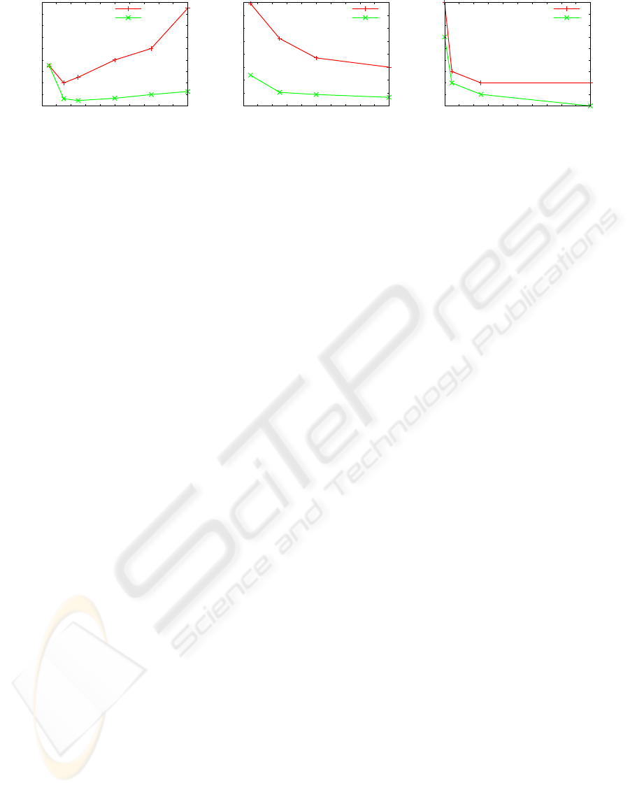
The inﬂuence of the size of the extracted subwin-

dows is signiﬁcant. In most of the cases, we observed

that there exist an optimal size, which is problem de-

pendent. This is illustrated for the Sowerby database

in Figure 2.

Concerning the number of trees, since each tree of

the ensemble classiﬁer is an independent realization

of the random tree growing process, the more trees

are grown, the better is the accuracy of the ensem-

ble classiﬁer. This is clearly illustrated in Figure 2 on

the Corel problem. In most cases, the error converges

however quite rapidly. With SCMMO, 10 trees give

already quite good results. Notice that more trees are

however needed with SCM since this latter does not

beneﬁt from the additional averaging effect of multi-

ple subwindows voting for a same pixel as in the case

of SCMMO.

Concerning the number of subwindows extracted

from the images in order to create the learning sam-

ple, like the number of trees, the larger it is, the better.

This is illustrated in Figure 2 in the case of the Retina

database. Notice that good results are typically ob-

tained by using a learning sample containing about

100 000 subwindows. Usually, this parameter should

be ﬁxed to the maximal possible value giventhe avail-

able computer resources.

The Extra-Tree parameter K inﬂuences both accu-

racy and computing times (lower values of K require

less score computations). Table 4 shows results in

terms of error rates and computing times for three val-

ues of K: K = 1, K =

√

m, and K = m, where m = 3wh

is the total number of attributes. Setting K to m im-

proves accuracy on Retina and Sowerby. The default

setting K =

√

m is however very close in terms of ac-

curacy and brings an important improvement of com-

puting times. Taking K = 1 deteriorates accuracy with

respect to the two other settings but the resulting error

FAST MULTI-CLASS IMAGE ANNOTATION WITH RANDOM SUBWINDOWS AND MULTIPLE OUTPUT

RANDOMIZED TREES

201

0 2 4 6 8 10 12 14 16 18 20

Error rate (%)

h(=w)

SCM

SCMMO

0 2 4 6 8 10 12 14 16 18 20

Error rate (%)

SCM

SCMMO

0 200 400 600 800 1000 1200 1400 1600 1800 2000

Error rate (%)

SCM

SCMMO

Figure 2: Left: error rate versus width (= height) of the subwindows on the Sowerby database. Middle: error rate versus

number of trees on the Corel database. Right: error rates versus total number of learning subwindows on the Retina database.

rate might still be considered acceptable for some ap-

plications where low computing times are important.

Note that this value of K amounts at building the trees

in an unsupervised way (ie., not looking at the outputs

when selecting the tests).

4 CONCLUSIONS AND FUTURE

WORK

In this paper, we have introduced and compared

two generic image annotation methods: SCM and

SCMMO. We have shown that the idea of (Mar´ee

et al., 2005) for image classiﬁcation using random

subwindows and ensemble of randomized trees can

be extended for pixel-wise labelling. In particular,

our extension of extremely randomized trees to deal

with multiple output prediction opens the door to a

wide range of potential applications. Indeed, from our

experiments on four distinct databases, SCMMO ap-

pears to be the most interesting one among the two

proposed methods: SCMMO is almost always signif-

icantly better than SCM and by using it, we obtained

good results on three problems among four. We deem

that the main merit of our approach is its good over-

all performance while remaining conceptually very

simple and keeping computing times very low. Our

approach also requires less tuning than others which

makes it an excellent candidate as an off-the-shelf

method even if it does not reach state-of-the-art re-

sults on each and every problem. Moreover, it might

be exploited as a ﬁrst, fast step for image annotation

as its output predictions might be post-processed by

various techniques at the local and/or global level.

Although we focused on the design of a generic

method, possible improvements or extensions of this

framework are numerous and might be considered to

improve results when dealing with a speciﬁc problem.

First, as proposed by (Mar´ee et al., 2005) in the con-

text of image classiﬁcation, it could be possible to in-

troduce more robustness into the pixel classiﬁcation

models by applying random perturbations (rotation,

scaling, etc.) to the subwindows or original images

before the learning stage. Computing features at mul-

tiple scales or orientations or over various ﬁlter re-

sponses (like in (Dollar et al., 2006)) instead of using

feature vectors composed by raw pixel values might

also help to achieve a higher level of invariance and

robustness to disturbances that might be required for a

given application. However, such an extension would

require additional computational costs.

There exist also several further degrees of free-

dom in the way subwindows are extracted. For in-

stance, we could generate several models exploit-

ing each a different size of input/output subwindows.

This would allow to combine into the ﬁnal model lo-

cal and global information from the images. For ex-

ample, some preliminary results show that combin-

ing three models built on subwindows of sizes 5 ×5,

2 × 30 and 30 × 2 reduces the error rate on Corel

dataset with SCMMO downto 33.89%. Optimizing

the number of models and the subwindow sizes might

further improve the accuracy on a given problem.

Also, our multiple output model can be cast as

a special case of the generic method proposed in

(Geurts et al., 2006b) to handle complex kernelized

output spaces. We believe that it would be interest-

ing to exploit this method with more ad hoc kernels

for image annotation, for example to take more ex-

plicitly into account correlations among neighboring

pixel classes or any other domain speciﬁc knowledge.

Comparison with other recent image annotation

methods using randomized trees should also be inves-

tigated (Shotton et al., 2008; Schroff et al., 2008).

Finally, other computer vision applications of ran-

dom subwindows and tree-based ensemble methods

with high-dimensionaloutput spaces might be investi-

gated, e.g. the detection of edges (Dollar et al., 2006).

ACKNOWLEDGEMENTS

PG and MD acknowledge the support of the Fonds

National de la Recherche Scientiﬁque (FNRS, Bel-

VISAPP 2009 - International Conference on Computer Vision Theory and Applications

202

gium). This paper presents research results of the

Belgian Network BIOMAGNET (Bioinformatics and

Modeling: from Genomes to Networks), funded by

the Interuniversity Attraction Poles Programme, initi-

ated by the Belgian State, Science Policy Ofﬁce. The

scientiﬁc responsibility rests with the authors.

REFERENCES

Amit, Y. and Geman, D. (1997). Shape quantization and

recognition with randomized trees. Neural computa-

tion, 9:1545–1588.

Bertelli, L., Byun, J., and Manjunath, B. S. (2007). A varia-

tional approach to exploit prior information in object-

background segregation: application to retinal images.

In ICIP.

Borenstein, E. and Malik, J. (2006). Shape guided object

segmentation. In CVPR, pages 969–976.

Bosch, A., Zisserman, A., and Munoz, X. (2007). Image

classiﬁcation using random forests and ferns. In Proc.

ICCV.

Breiman, L., Friedman, J., Olshen, R., and Stone, C. (1984).

Classiﬁcation and Regression Trees. Wadsworth and

Brooks, Monterey, CA.

Cour, T. and Shi, J. (2007). Recognizing objects by piecing

together the segmentation puzzle. In CVPR.

Dollar, P., Tu, Z., and Belongie, S. (2006). Supervised

learning of edges and object boundaries. In CVPR,

pages 1964–1971.

Dumont, M., Mar´ee, R., Wehenkel,

L., and Geurts, P. (2009).

http://www.monteﬁore.ulg.ac.be/services/stochastic/

pubs/2009/DMWG09/.

Ernst, D., Mar´ee, R., and Wehenkel, L. (2006). Reinforce-

ment learning with raw image pixels as input state.

In Proc. International Workshop on Intelligent Com-

puting in Pattern Analysis/Synthesis, volume 4153 of

Lecture Notes in Computer Science, pages 446–454.

Geurts, P., Ernst, D., and Wehenkel, L. (2006a). Extremely

randomized trees. Machine Learning, 36(1):3–42.

Geurts, P., Wehenkel, L., and d Alch´e-Buc, F. (2006b). Ker-

nelizing the output of tree-based methods. In ICML,

pages 345–352.

He, X., Zemel, R., and Carreira-Perpinan, M. (2004). Mul-

tiscale conditional random ﬁelds for image labelling.

In CVPR, volume 2, pages 695–702.

He, X., Zemel, R., and Ray, D. (2006). Learning and in-

corporating top-down cues in image segmentation. In

ECCV, pages 338–351.

Jodogne, S., Briquet, C., and Piater, J. (2006). Approxi-

mate policy iteration for closed-loop learning of vi-

sual tasks. In Proc. of the 17th European Conference

on Machine Learning, volume 4212, pages 222–226.

Lepetit, V. and Fua, P. (2006). Keypoint recognition us-

ing randomized trees. IEEE Transactions on Pattern

Analysis and Machine Intelligence, 28(9):1465–1479.

Mar´ee, R., Geurts, P., Piater, J., and Wehenkel, L. (2005).

Random subwindows for robust image classiﬁcation.

In CVPR, volume 1, pages 34–40.

Mar´ee, R., Geurts, P., Visimberga, G., Piater, J., and We-

henkel, L. (2003). An empirical comparison of ma-

chine learning algorithms for generic image classiﬁ-

cation. In Proc. SGAI-AI, pages 169–182.

Mar´ee, R., Geurts, P., and Wehenkel, L. (2007). Content-

based image retrieval by indexing random subwin-

dows with randomized trees. In Proc. ACCV, volume

4844 of LNCS, pages 611–620.

Meurie, C., Lebrun, G., Lezoray, O., and Elmoataz, A.

(2003). A comparison of supervised pixels-based

color image segmentation methods. application in

cancerology. WSEAS Transactions on computers, spe-

cial issue on SSIP’03, 2:739–744.

Moosmann, F., Triggs, B., and Jurie, F. (2006). Randomized

clustering forests for building fast and discriminative

visual vocabularies. In Neural Information Processing

Systems (NIPS).

Nowak, E. and Jurie, F. (2007). Learning visual similarity

measures for comparing never seen objects. In Proc.

IEEE CVPR.

Nowak, E., Jurie, F., and Triggs, B. (2006). Sampling strate-

gies for bag-of-features image classiﬁcation. In Proc.

ECCV, pages 490–503.

Philbin, J., Chum, O., Isard, M., Sivic, J., and Zisserman, A.

(2007). Object retrieval with large vocabularies and

fast spatial matching. Proc. IEEE CVPR.

Schroff, F., Criminisi, A., and Zisserman, A. (2008). Object

class segmentation using random forests. In Proc. of

the British Machine Vision Conference (BMVC).

Shotton, J., Johnson, M., and Cipolla, R. (2008). Semantic

texton forests for image categorization and segmenta-

tion. In Proc. IEEE Conference on Computer Vision

and Pattern Recognition (CVPR).

Shotton, J., Winn, J., Rother, C., and Criminisi, A. (2006).

Textonboost: Joint appearance, shape and context

modeling for multi-class object recognition and seg-

mentation. In ECCV, pages I: 1–15.

Shotton, J., Winn, J., Rother, C., and Criminisi, A. (2007).

Textonboost for image understanding: Multi-class ob-

ject recognition and segmentation by jointly modeling

appearance, shape and context. In International Jour-

nal on Computer Vision.

Verbeek, J. and Triggs, B. (2007). Scene segmentation with

conditional random ﬁelds learned from partially la-

beled images. In Proc. NIPS.

Yin, P., Criminisi, A., Winn, J., and Essa, I. (2007). Tree-

based classiﬁers for bilayer video segmentation. In

Proc. CVPR.

Yu, S. X. and Shi, J. (2003). Object-speciﬁc ﬁgure-ground

segregation. In CVPR, volume 2, pages 39–45.

FAST MULTI-CLASS IMAGE ANNOTATION WITH RANDOM SUBWINDOWS AND MULTIPLE OUTPUT

RANDOMIZED TREES

203