INSCRIBED CONVEX SETS AND DISTANCE MAPS

Application to Shape Classiﬁcation and Spatially Adaptive Image Filtering

erique Robert-Inacio

IM2NP - UMR CNRS 6242, ISEN-Toulon, Place Pompidou, Toulon, France

Keywords:

Distance map, Inscribed convex set, Shape classiﬁcation, Similarity parameter, Spatially adaptive ﬁltering.

Abstract:

This paper presents two original applications related to discrete distance maps. Based on the relation linking

inscribed convex sets and discrete distance maps, the ﬁrst application is a spatially adaptive ﬁltering method

which is set up for both grey-level and color images. This spatially adaptive ﬁlter is really efﬁcient in perfor-

mances and computation time. Furthermore a new mean of computation for the Asplund distance as well as

a method for determining the similarity degree between shapes are also presented. The similarity parameter

enables a quantitative shape classiﬁcation with respect to a set of reference shapes.

1 INTRODUCTION

The discrete distances are widely used in image pro-

cessing. For example, they can be used to determine

Vorono

ı diagram around objects or the medial axis

and skeleton of a shape and so on, as well as they can

achieve elementary morphological operations such as

dilation or erosion (Soille, 1999)(Borgefors et al.,

1999) in 2D or in 3D. But another kind of information

in relation with inscribed convex sets can be extracted

from distance maps.

This paper deals with two of the applications in-

volving inscribed convex sets: on the one hand, a spa-

tially adaptive ﬁlter is set up by determining a cus-

tomized ﬁltering window size at each point of an im-

age in grey-levels or in color, and on the other hand,

a simpliﬁed method for the determination of the As-

plund distance and of a degree of similarity between

shapes is described.

2 DISCRETE DISTANCE MAPS

A discrete distance map (DDM) is computed from a

binary image including a background and one or sev-

eral objects. On the DDM, the distance to the nearest

object is estimated at each point of the background

and each point of the object set is set to 0. There exist

several algorithms evaluating the Euclidean distance

in a discrete space (Danielsson, 1980). But several

works presented discrete distances on Z

as approxi-

mations of the Euclidean distance, as described in the

following section.

2.1 Approximation of the Euclidean

Distance

At the beginning, discrete distances such as Man-

hattan distance or chessboard distance, were deﬁned

in order to coarsely estimate the Euclidean distance

between points on a grid (Rosenfeld and Pfaltz,

1968)(Borgefors, 1986). These approximations were

reﬁned by the elaboration of the chamfer distances.

Let us deﬁne the discrete distances.

Let A(x

, y

) and B(x

, y

) be two points of Z

The Manhattan distance is deﬁned by:

(A, B) = |x

− x

| + |y

− y

| (1)

The chessboard distance is deﬁned by:

(A, B) = max (|x

− x

|, |y

− y

|) (2)

Notice that d

(A, B) ≥ d

(A, B), ∀(a, B) ∈ Z

A family of discrete distances called chamfer dis-

tances also gives an approximation of the Euclidean

distance. The principle of computation for such dis-

tances is based on the determination of a minimal path

leading from A to B. This path is made of several ele-

mentary displacements, each of them being weighted.

Examples of weights for the main directions on the

grid are given in Fig. 1 and the corresponding estima-

tions of Euclidean distance values are given in Table

Robert-Inacio F. (2009).

INSCRIBED CONVEX SETS AND DISTANCE MAPS - Application to Shape Classiﬁcation and Spatially Adaptive Image Filtering.

In Proceedings of the Fourth International Conference on Computer Vision Theory and Applications, pages 60-66

DOI: 10.5220/0001796200600066

 SciTePress

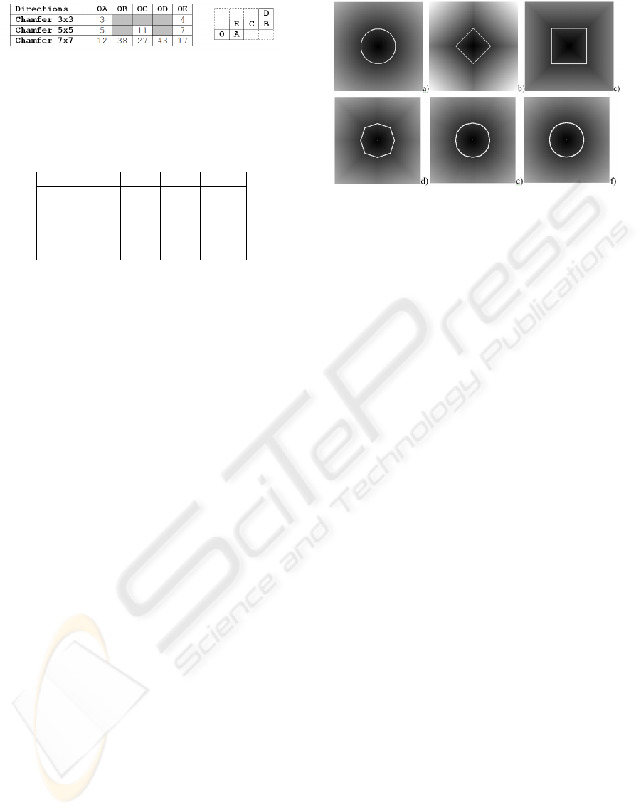
Figure 1: Weights and elementary displacements for the

chamfer distances with a neighborhood width of 3, 5 and

Table 1: Distances from O for the chamfer distance with

different neighborhood widths.

Point/Width 3 5 7

A 1 1 1

B 10/3 16/5 19/6

C 7/3 11/5 9/4

D 11/3 18/5 43/12

E 4/3 7/5 17/12

The previous examples can be extended to an arbi-

trary dimension of neighborhood, in order to be more

accurate in the estimation of the Euclidean distance,

with the main drawback that it makes the computation

time increase.

2.2 Associated Convex Sets

Fig. 2 shows DDM computed from a binary image

containing a unique object: the center point. DDM

are given for the Euclidean distance and the discrete

distances deﬁned above. Furthermore sets of equidis-

tant points to the object set at a distance of 50 are

drawn in white in Fig. 2. If we consider that the cir-

cle C

(M, R) of center M and radius R, is the set of

equidistant points from M at a Euclidean distance of

R, then, by extension, sets of white points of Fig. 2

are ”circles” of radius 50 for the corresponding dis-

tances. In this way, we can associate the shape of

these ”circles” with the corresponding distance. Ta-

ble 2 summarizes the correspondence. Note that all

of these shapes are regular. Fig. 3 presents an exam-

ple of inscribed ”circles” into a particular shape.

3 INSCRIBED CONVEX SETS

By deﬁnition a DDM gives at each point x of the

background its distance to the nearest object. In the

Euclidean case, if DDM(x) is the value reached at

point x, the disk D(x, DDM(x)) of center x and radius

DDM(x) is totally included in the background. Fur-

thermore DDM(x) is the distance from x to the object

set. That means that D(x , DD(x)) is the greatest disk

centered at x and totally included in the background.

This remark can be generalized to the convex sets as-

sociated with the discrete distances deﬁned above. In

Figure 2: DDM for a) the Euclidean distance, b) the Man-

hattan distance, c) the chessboard distance, d) the 3x3

chamfer distance, e) the 5x5 chamfer distance and f) the

7x7 chamfer distance.

this way if X is the shape corresponding to a discrete

distance, X(x, DDM(x)) is the greatest homothetic set

of X centered at x and totally included in the back-

ground.

Let us now consider a set Y and compute a par-

ticular DDM by considering the outside of Y (or its

complementary set) as the object and Y as the back-

ground. The maximum value, DDM(x

max

), reached

on the DDM gives the scale ratio corresponding to an

inscribed set of shape X into Y . Thus, DDM(x

max

) is

the scale ratio applied to the shape X to obtain the in-

scribed homothetic set of X into Y , if we consider that

X is the reference shape at scale 1. Depending on the

shape Y , x

max

is unique or not, in other words, there

can exist several positions to center the inscribed ho-

mothetic set of X into Y .

4 SPATIALLY ADAPTIVE

FILTERING

4.1 Adaptive Sliding Window Size

Sliding windows used for ﬁltering are generally

square-shaped and these squares are oriented at 0

But such squares are ”circles” for the chessboard dis-

tance. That is why we are going to use a DDM based

on the chessboard distance to design the sliding win-

dow associated with a given point. As the chess-

board DDM allows to determine the greatest homo-

thetic square totally included in the background, it is

sufﬁcient to compute an appropriate binary image de-

scribing objects and background, in order to obtain

window sizes depending on the location and stored in

the DDM.

For grey-level images, the binary image can be

chosen as a thresholded gradient image (TG). In this

INSCRIBED CONVEX SETS AND DISTANCE MAPS - Application to Shape Classification and Spatially Adaptive

Image Filtering

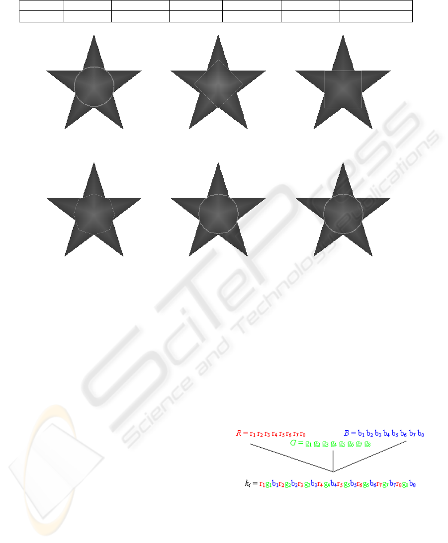
Table 2: Correspondance between discrete distances and associated convex shapes.

Distance Euclidean Manhattan Chessboard Chamfer 3x3 Chamfer 5x5 Chamfer 7x7

Shape Circle Square (45

) Square (0

) Octagon Dodecagon 24-edge Polygon

a b c

d e f

Figure 3: Inscribed ”circles” for a) Euclidean, b) Manhattan, c) Chessboard, d) Chamfer 3x3, e) Chamfer 5x5 and f) Chamfer

7x7 distances.

way high frequency areas are preserved while homo-

geneous regions are smoothed. The threshold value is

chosen by taking into account the maximal amplitude

of noise that must be ﬁltered.

For color images, we compute a color distance

map (CDM) that will be thresholded. This CDM is

derived from two color difference images. In other

words, the Euclidean distance between the color vec-

tor of point P(x , y) and those of its right neighbor

(x + 1, y) is computed on the original color image

to obtain the X-CDM. As well, the Y-CDM is ob-

tained by computing the Euclidean distance between

the color vector of P(x, y) and those of its top neigh-

bor P

(x, y + 1). A threshold value v is then chosen

according to the amplitude of noise to be ﬁltered. Ac-

tually noise of amplitude lower or equal to th will be

removed whereas noise of greater amplitude will be

consider as relevant information. Thus the X-CDM

and Y-CDM are thresholded at v and the thresholded

CDM is obtained by mixing these two binary images

in order to keep all data representing high color dis-

tances.

Then the chessboard DDM is computed from one

of those binary images by considering points of high

frequency or of high color distance as the object set.

In this way, at each point of the background, the DDM

gives the half width of the maximal square totally in-

cluded in the background. If ww(P) is the maximal

window width at point P(x, y), ww(P) depends on the

location of P and it is the adaptive size of the sliding

window and:

∀P(x, y) ∈ Z

, ww(P) = 2 × DDM(P) + 1 (3)

Figure 4: Bit-mixing paradigm.

4.2 Median Filter

For grey-level images the median ﬁlter is achieved by

determining the median value for each sliding win-

dow. Let us note that a sliding window contains

ww(P)

points and that this number is an odd value.

Grey-level values belonging to a sliding window are

VISAPP 2009 - International Conference on Computer Vision Theory and Applications

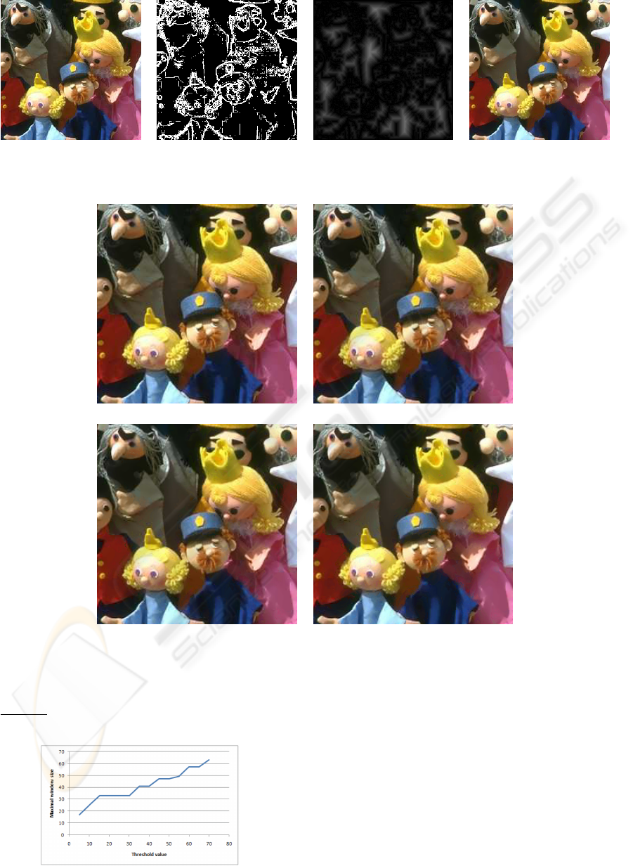
a b c d

Figure 5: Adaptive median ﬁltering process: a) original image, b) thresholded CDM, c) chessboard DDM, d) ﬁltered image.

a b

c d

Figure 6: Adaptive median ﬁltering results for different values of th: a) th = 5, b) th = 10, c) th = 20, d) th = 30.

sorted and the median value is determined as the



ww(P)



one.

Figure 7: Maximal window size according to th.

For color images (Robert-Inacio and Dinet, 2006),

it is not possible to sort color vectors as they belong

to Z

which does not have total order. So a bit-

mixing paradigm (Lambert and Macaire, 2000)(Fig.

4) is used in order to associate a 24-bit integer value

(r, g, b) to each RGB color vector (r, g, b). In this

way it is possible to arrange in order color vectors of

the sliding window according to their v

(r, g, b), and

then, to determine the median value. This way to sort

colors can be unsatisfactory from a theoretical point

of view, but it gives efﬁcient results in practice. Fig.

5 shows the whole process on a color image.

INSCRIBED CONVEX SETS AND DISTANCE MAPS - Application to Shape Classification and Spatially Adaptive

Image Filtering

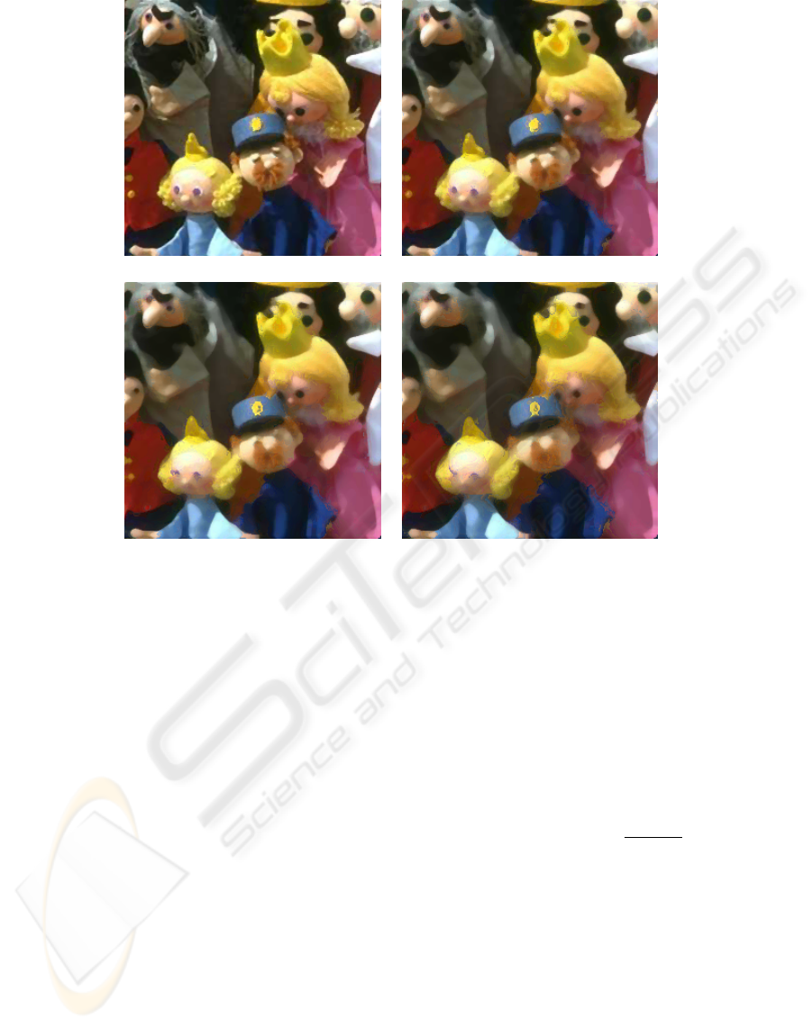
a b

c d

Figure 8: Median ﬁltering results for different window widths: a) 3x3, b) 5x5, c) 7x7, d) 9x9.

4.3 Experimental Results

Fig. 6 shows ﬁltered images obtained for 4 differ-

ent threshold values of the CDM. We can note that

some degradation in hair areas. The maximal size for

sliding windows is respectively of 17, 25, 33 and 33

for th = 5, 10, 20 or 30. Fig. 7 shows the evolution

of the maximal window size according to the thresh-

old value of the CDM, for this particular image. The

higher th, the smoother the result, with the drawback

of loosing relevant information. Fig. 8 shows the

rapid degradation of the ﬁltered image in case of ﬁxed

window size on the whole image.

5 SHAPE CLASSIFICATION

Shape classiﬁcation can be achieved by using qual-

itative or quantitative tools. In the second case, the

classiﬁcation is made with respect to one or several

criteria. In order to do that, shape parameters or dis-

tance between shapes can be used. In this section,

we recall the deﬁnition of the Asplund distance be-

tween shapes and of a similarity parameter estimating

the degree of likeliness of the shape under study to a

reference shape.

5.1 Asplund Distance

The Asplund distance (Serra, 1988)(Robert-Inacio,

2007) between two compact sets X and Y of R

(X,Y ), is deﬁned by:

(X,Y ) = ln

k(X,Y )

K(X,Y )

(4)

where:

k(X,Y ) = in f {k > 0,Y ⊂

k.X} (5)

K(X,Y ) = sup{k > 0, k.X ⊂

Y } (6)

⊂

means that it exists x ∈ R

such that x + X ⊂

Y . In other words, k(X,Y ) is the scale ratio so that

k(X,Y ).X is circumscribed to Y and K(X ,Y ) is the

scale ratio so that K(X,Y ).X is inscribed into Y . We

can also remark that:

K(X,Y ) = k(Y, X) (7)

VISAPP 2009 - International Conference on Computer Vision Theory and Applications

5.2 Similarity Parameter

The similarity parameter SP is deﬁned for any pair of

convex sets X and Y of R

by the following formula

(Robert, 1998)(Robert-Inacio, 2007):

SP(X,Y ) =

k(X,Y )

k(Y, X)

µ(X)

µ(Y )

(8)

where µ is the surface area measure.

5.3 Implementation

In this section, let us consider the case where X is a

”circle” for a discrete distance. It is then very easy to

determine the ratio to inscribe X into Y , by computing

the corresponding DDM inside Y . In this case, the

maximal value is k(X,Y ).

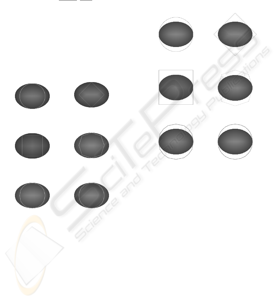
a b

c d

e f

Figure 9: Inscribed ”circles” for a) Euclidean, b) Manhat-

tan, c) Chessboard, d) Chamfer 3x3, e) Chamfer 5x5 and f)

Chamfer 7x7 distances.

DDM can also be useful in the particular case

where Y is symmetrical with respect to a point c. In

this case the center point c is the center of the homo-

thetic set of X , circumscribed to Y . It is then sufﬁ-

cient to compute another DDM by considering a set

object reduced to c, DDM(c). And the maximal value

reached on the boundary of Y by DDM(c) is the scale

ratio to apply to X (shape at scale 1) so that it is cir-

cumscribed to Y . In other cases algorithms such that

the circumscribed disk algorithm and its extension to

convex sets must be used. Fig. 9 and 10 illustrate the

computation of inscribed and circumscribed convex

sets X in the case where Y is convex and symmetrical.

We can note that the circumscribed disk algorithm

and its extension to convex sets and the DDM can be

extended to the third dimension (Jones et al., 2006).

Furthermore other distance maps can generate other

”circles” and then comparison to these new shapes

can be achieved (Strand et al., 2006).

a b

c d

e f

Figure 10: Circumscribed ”circles” for a) Euclidean, b)

Manhattan, c) Chessboard, d) Chamfer 3x3, e) Chamfer 5x5

and f) Chamfer 7x7 distances.

6 CONCLUSIONS

Applications involving discrete distance maps are nu-

merous and most of them are related to mathemati-

cal morphology. In this paper we have presented a

spatially adaptive median ﬁlter using discrete distance

maps in order to determine the greatest size of sliding

window at each point of the image. This ﬁlter enables

a better smoothing of quite homogeneous areas while

preserving regions where gradient or color distance is

relevant. This method gives satisfactory results.

In a second time, we have described an application re-

lated to shape classiﬁcation. Discrete distance maps

can be used in this case, if one of the shapes to com-

pare is a ”circle” for a given discrete distance. In this

way, the computation of the inscribed shape into the

other one is simpliﬁed as it is achieved by determining

the maximal value on the corresponding discrete dis-

INSCRIBED CONVEX SETS AND DISTANCE MAPS - Application to Shape Classification and Spatially Adaptive

Image Filtering

tance maps. The circumscribed shape can also be de-

termined from a particular discrete distance map if the

other shape is symmetrical. Furthermore results con-

cerning shape classiﬁcation can be easily extended to

the 3D.

REFERENCES

Borgefors, G. (1986). Distance transformations in digital

images. CVGIP, 34:344–371.

Borgefors, G., Nystrom, I., and SannitiDiBaja, G. (1999).

Computing skeletons in three dimensions. Pattern

Recognition, 32:1225–1236.

Danielsson, P. (1980). Euclidean distance mapping.

CVGIP, 14:227–248.

Jones, M., Baerentzen, J., and Sramek, M. (2006). 3d dis-

tance ﬁelds: a survey of techniques and applications.

IEEE trans. on visualization and computer graphics,

12/4:581–599.

Lambert, P. and Macaire, L. (2000). Filtering and segmen-

tation : the speciﬁcity of color images. In Conference

on Color in Graphics and Image Processing, pages

57–64, Saint-Etienne, France.

Robert, F. (1998). Shape studies based on the circumscribed

disk algorithm. In IEEE-IMACS, CESA 98, pages

821–826, Hammamet, Tunisia.

Robert-Inacio, F. (2007). A relation between a similarity

parameter, the asplund distance and discrete distance

maps. In IVCNZ 2007, pages 254–259, Hamilton,

New Zealand.

Robert-Inacio, F. and Dinet, E. (2006). An adaptive median

ﬁlter for colour image processing. In 3rd CGIV, pages

205–210, Leeds, UK.

Rosenfeld, A. and Pfaltz, J. (1968). Distance functions in

digital pictures. Pattern Recognition, 1:33–61.

Serra, J. (1988). Image analysis and mathematical mor-

phology: theoretical advances. Academic Press.

Soille, P. (1999). Morphological image analysis. Springer

Verlag, Berlin.

Strand, R., Nagy, B., Fouard, C., and Borgefors, G. (2006).

Generating distance maps with neighbourhood se-

quences. In DGCI 2006, volume 4245, pages 295–

307, Szeged, Hungary.

VISAPP 2009 - International Conference on Computer Vision Theory and Applications