WELDING INSPECTION USING NOVEL SPECULARITY
FEATURES AND A ONE-CLASS SVM
Fabian Timm, Sascha Klement, Thomas Martinetz and Erhardt Barth
Institute for Neuro- and Bioinformatics, University of Luebeck, Ratzeburger Allee 160, Luebeck, Germany
Keywords:
Feature extraction, One-class classification, Welding seam inspection, Machine vision.
Abstract:
We present a framework for automatic inspection of welding seams based on specular reflections. Therefore,
we introduce a novel feature set – called specularity features (SPECs) – describing statistical properties of
specular reflections. For classification we use a one-class support-vector approach. The SPECs significantly
outperform statistical geometric features and raw pixel intensities, since they capture more complex charac-
teristics and depencies of shape and geometry. We obtain an error rate of 9%, which corresponds to the level
of human performance.
1 INTRODUCTION
In many industrial processes individual parts are
joined by using welding techniques. Soldering and
welding techniques are common in diverse areas such
as printed circuit board assembly or automotive line
spot welding. The quality of a single welding often
defines the grade of the whole product, for example
in critical areas such as automotive or aviation indus-
try, where failures of the welding process can cause
a malfunction of the whole product. Typically, welds
are made by a laser or a soldering iron. During the last
few years lasers and their usage in industrial appli-
cations have become affordable for many companies.
Although the initial cost of a laser-welding system is
still high, their wearout is low and so the service inter-
vals are very long. A laser weld is more precise than
a weld by a soldering iron, but the quality can also
vary due to shifts of the part towards the laser or due
to material impurities. Therefore, an inspection of the
welding is required in order to guarantee an accurate
quality.
There are several machine vision approaches to
automatically classify the quality of solder joints.
These approaches can be divided into two groups.
The first group deals with special camera and lighting
setups to gain the best image representation of the rel-
evant features (Ong et al., 2008; Kim and Cho, 1995;
Chiu and Perng, 2007). In the second group, the cam-
era and lighting setup is often predetermined and the
inspection is done by sophisticated pattern recogni-
tion methods. In the last few years several approaches
for automatic inspection of solder joints concerning
feature extraction, feature selection, and classifica-
tion were proposed (Ko and Cho, 2000; Poechmueller
et al., 1991; Ong et al., 2008; Driels and Lee, 1988;
Kim and Cho, 1995). Like in many other appli-
cations, neural networks and especially the support-
vector-machine have become state-of-the-art (Cortes
and Vapnik, 1995; Boser et al., 1992; Vapnik, 1995).
In this work we focus on the inspection of cath-
odes welded by an Nd:YAG (neodymium-doped yt-
trium aluminium garnet) laser during the production
of lamps. Due to its position in the whole production
process, the camera and lighting setup was fixed and
could not be changed. Since the welded cathode has
specific specular reflections, an appropriate feature
extraction is required in order to achieve an accurate
performance. Therefore, we introduce a novel feature
set called specularity features (SPECs). The SPECs
contain statistics of certain shape characteristics of
single components and can cover a wide range of
complex shape properties and their dependencies. For
the classification we use a one-class support-vector
approach (Sch
¨
olkopf et al., 2001; Tax and Duin, 2004;
Labusch et al., 2008) in order to describe features of
accurate weldings and to separate them from all other
possible inaccurate weldings. We also evaluate those
SPECs that are most relevant for the classification and
compare them to the physical shape of the cathode.
For comparison we use raw pixel intensities and
the statistical geometric feature (SGF) algorithm
which computes simple geometric characteristics of
binary components.
146
Timm F., Klement S., Barth E. and Martinetz T.
WELDING INSPECTION USING NOVEL SPECULARITY FEATURES AND A ONE-CLASS SVM.
DOI: 10.5220/0001776301450152
In Proceedings of the Fourth International Conference on Computer Vision Theory and Applications (VISIGRAPP 2009), page
ISBN: 978-989-8111-69-2
Copyright
c
 2009 by SCITEPRESS – Science and Technology Publications, Lda. All rights reserved

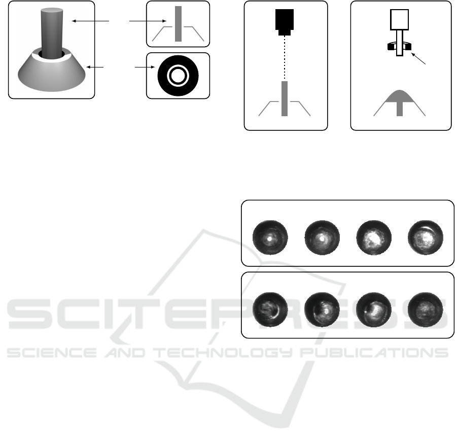
pin
socket
Figure 1: A 3d drawing of the cathode (left), a cross-section
(upper right) and the image of the camera are shown (lower
right).
In section 2 we give a brief overview of the camera
and lighting setting and the image acquisition. The
methods for feature extraction and classification are
described in section 3. Experiments and the results
are shown in section 4. We conclude with a discussion
in section 5.
2 IMAGE ACQUISITION
An unwelded cathode consists of a socket and a pole
that may be composed of different materials (see
Fig. 1). In a top view with directional parallel light
the unwelded cathode simplifies to only four compo-
nents – two black rings (the slant of the neck and the
space between pin and socket), one white ring (neck
of the socket) and one white circle (top of the pin, see
Fig. 1 bottom right). Hence, a component analysis of
the grey value image of the welded cathode can be
used to extract specific features.
A correct combination of camera, lens and illu-
mination is very important to achieve the best perfor-
mance in classification. However, sometimes the best
setup can not be chosen due to limited space or other
requirements. For this work, there was only one cam-
era setup practicable (see Fig. 2). We used a standard
analog monochrome VGA video camera, a single-
sided telecentric lens and a LED ring light with a Fres-
nel lens. We collected 934 images containing 657 im-
ages of non-defective cathodes and 277 images of de-
fective cathodes. All images were labelled by experts,
scaled to unit size (96 × 96 pixel) and smoothed by a
Gaussian filter (5×5, σ = 1). The unwelded cathodes
are first separated by a simple template matching such
that the dataset contains images of welded cathodes.
Moreover, the dataset only consists of images which
are difficult to classify manually.
Since defective cathodes are determined by the
mean time to failure, the true class labels are not
known in general. Therefore, the experts look for
aberrations that were selected by extensive bench-
laser
lens
ring light
camera
Figure 2: Drawing of the setup for laser welding (left) and
image acquisition (right). The laser and the camera are lo-
cated on top of the cathode. The distance between the LED
ring light and the cathode is chosen such that angle of inci-
dence is very small.
no defects
defects
Figure 3: Example images of cathodes (top row) and defec-
tive cathodes (bottom row).
mark tests. Example images of defective and non-
defective cathodes are shown in Fig. 3. The reflec-
tions of cathodes without a defect vary due to dif-
ferences in material and position of the pin. Also,
a slight deflection of the pin just before the welding
can affect the quality of the welding. Some of the de-
fective cathodes have holes caused by a slanted pin,
others do not have any reflections due to a very rough
surface. Therefore, the variety of defects can not be
described easily, and a feature extraction method that
covers several geometric properties and complex de-
pendencies between components is required.
3 METHODS
Recently, several approaches for the inspection of sol-
der joints were proposed (Ong et al., 2008; Chiu and
Perng, 2007; Ko and Cho, 2000; Kim and Cho, 1995;
Driels and Lee, 1988). Some of these methods com-
pute simple features in a manually tiled binary image,
others use the pixel intensities directly as input fea-
WELDING INSPECTION USING NOVEL SPECULARITY FEATURES AND A ONE-CLASS SVM
147

tures for a neural network or a support vector machine
(Cortes and Vapnik, 1995; Boser et al., 1992; Vap-
nik, 1995). Hence, the preprocessing often involves
a considerable downsampling of the images in order
to reduce the dimensionality. Usually, this downsam-
pling reduces the information of the images and yields
poor error rates. A better performance is achieved by
extracting specific features that describe the relevant
reflections of the weldings.
In this work, we present a novel approach for
the extraction of specularity features called SPECs.
These features describe several complex properties of
specular reflections and their dependencies. For com-
parison we also use the statistical geometric feature
(SGF) approach as well as raw pixel intensities.
In the following, we will describe the extraction of
SGFs and SPECs. Since the images were recorded by
an 8bit monochrome camera, we focus on grey value
images, but the approach can easily be extended to
colour images.
3.1 Statistical Geometric Features
Originally, SGFs were used for texture classifica-
tion with 16 features for each image (Chen et al.,
1995). Further extensions were developed for cell nu-
clei classification and contained 48 features (Walker
and Jackway, 1996). SGFs compute simple shape
properties of local components. Hence, they can be
used to extract specific features of welding images.
Moreover, SGFs are very intuitive and computed effi-
ciently.
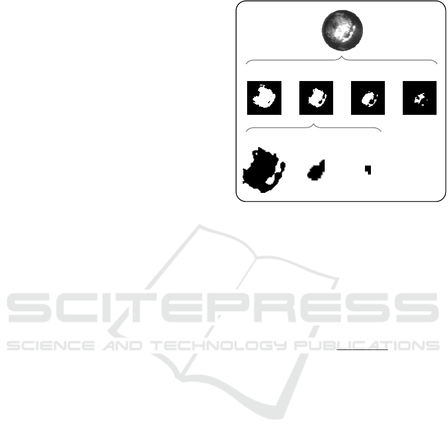
For each l-bit grey value image I a stack of binary
images B = {I
τ
} with τ ∈{1, 2, 3,...,2
l
} is generated.
A single binary image I
τ
is computed such that
I
τ
(x,y) =

1 : I(x, y) ≥ τ
0 : I(x, y) < τ
.
(1)
This decomposition is lossless, since the input im-
age can always be recovered by summing up all bi-
nary images. Furthermore, each binary image I
τ
is de-
composed into a set of black and white components,
{C
0
(τ),C
1
(τ)}with C
0
(τ) = {C
(0,τ)
1
,...,C
(0,τ)
m
}, and
C
1
(τ) =

C
(1,τ)
1
,...,C
(1,τ)
n

, respectively (see Fig. 4).
The subscript 0 denotes a black component and the
subscript 1 a white component.
Each component C
( j,τ)
i
= {~x
k
} consists of pixel
positions ~x
k
∈ {1,2, ..., H}×{1, 2,...,W }, where H
and W are the height and the width of the input image.
For convenience we omit the indices of a component
if they are not necessary. We also use C
i
= C
( j,τ)
i
for
abbreviation.
The area of a component equals the number of its
··· ··· ···
I
τ
1
I
τ
k
input image I
C
(1,τ)
1
C
(0,τ)
1
C
(0,τ)
2
Figure 4: Decomposition scheme for a grey value input im-
age. First, the input image (first row) is decomposed into
several binary images I
τ
(second row). Afterwards each
binary image is further separated into its black and white
components (third row). The white component C
(1,τ)
1
is in-
verted, for convenience.
pixels,
AREA (C) = card (C) . (2)
The relative size of a single component C
i
with re-
spect to all components is defined as
PROP (C
i
) =
AREA (C
i
)
∑
k
AREA (C
k
)
. (3)
Based on the stack of binary images, the feature
extraction of the SGF algorithm can be divided into
two stages – a local stage and a global stage. In the lo-
cal stage several features for each component are cal-
culated (see Tab. 1). A single binary image is then de-
scribed by a set of averaged shape and position prop-
erties of all black and white components.
In the second stage the local features are com-
bined to global features using first order statistics (see
Tab. 2). In total, the SGF algorithm determines 48
features for a single input image.
3.2 Specularity Features (SPEC)
Since the statistical geometric features were mainly
developed for classification of textures, i.e. repeti-
tive patterns, they are not suitable for the inspection of
welding seams, which usually do not have a repetitive
structure. Instead, properties that describe the char-
acteristic shapes of specular reflections are required.
For example, some defective cathodes have long nar-
row reflections at the neck of the socket which can
VISAPP 2009 - International Conference on Computer Vision Theory and Applications
148

Table 1: Local features for a single binary image I
τ
of size H ×W (Walker and Jackway, 1996).
description formula
number of black/white components NOC(τ) = |C(τ)|
averaged irregularity IRGL (τ) =
∑
k
IRGL(C
k
) AREA(C
k
)
∑
k
AREA(C
k
)
averaged clump displacement DISP(τ) =
1
NOC(τ)
∑
k
DISP(C
k
)
averaged clump inertia INERTIA(τ) =
1
NOC(τ)
∑
k
DISP(C
k
)AREA(C
k
)
total clump area TAREA(τ) =
1
H W
∑
k
AREA(C
k
)
averaged clump area CAREA
i
(τ) =
1
NOC(τ)
∑
k
AREA(C
k
)
where
IRGL (C) =
1 +
√
π max
~x∈C
k~x −~µ(C)k
p
AREA(C)
−1 is the irregularity of the component C,
DISP(C) =
√
π
k
~µ(C) −~µ
I
k
√
H W
is the relative displacement of the component C,
~µ(C) is the centre of gravity of the component C and~µ
I
is the centre of the image.
be covered by features such as the formfactor and the
extent.
We make use of the general decomposition
scheme of binary images and evaluate appropriate
features covering the properties of specular reflec-
tions. We compute several general properties of each
component (see Tab. 3). Using a 4-neighbourhood
two successive boundary points are denoted by~x
m
and
~x
m+1
, F(α) is the maximum distance between two
boundary points when rotating the coordinate axis by
α ∈ A = {0
◦
,5
◦
,..., 175
◦
}, w
BR
and h
BR
are the width
and height of the bounding rectangle and a, b are the
major and minor axis of the ellipse that has the same
second moments as the region. For a detailed dis-
cussion on geometric shapes see chapter 9 of (Russ,
2007).
Table 2: Global features. f is one of the local features de-
scribed before.
maximum = max
τ
f (τ)
mean =
1
|τ|
∑
τ
f (τ)
sample mean =
1
∑
τ
f (τ)
∑
τ
τ f (τ)
sample std. =
v
u
u
u
u
t
∑
τ
(τ −sample mean)
2
f (τ)
∑
τ
f (τ)
The local features are computed for each compo-
nent and need to be combined to form a single feature.
Hence, we scale each feature in two different ways.
First, we calculate the mean weighted by the relative
size of the components, and second, we scale the sum
by the total number of components. For example, for
the averaged perimeter of the binary image I
τ
these
two scalings are:
PERIM(τ) =
∑
k
PERIM(C
k
) PROP(C
k
) , (4)
PERIM(τ) =
1
NOC(τ)
∑
k
PERIM(C
k
) , (5)
where PROP(C
k
) is defined in Eq. 3. Using these
scalings two aspects can be covered simultaneously.
On the one hand, if small reflections are important,
they are considered by scaling with the number of
components. On the other hand, if large reflections
are relevant, they become important when scaling by
the relative size.
We combine the local features by computing
minimum, variance, median, and entropy besides
the statistics of Tab. 2. Whereas the sample mean and
sample std. range over the threshold τ, the new fea-
tures are statistics over local shape features. Hence,
we can, for example, evaluate the variance of the
number of white components or the entropy of the
formfactor of white components. Moreover, extreme
shape properties of components become less impor-
tant when using the median.
In total, for a single image, we determine 768 fea-
tures consisting of:
WELDING INSPECTION USING NOVEL SPECULARITY FEATURES AND A ONE-CLASS SVM
149

Table 3: Features for a component C.
perimeter:
PERIM(C) =
N−1
∑
m=1
k~x
m
−~x
m+1
k
2
maximum Feret diameter:
MAXFD(C) = max
α∈A
F(α)
minimum Feret diameter:
MINFD(C) = min
α∈A
F(α)
mean Feret diameter:
MEANF(C) =
1
|A|
∑
α∈A
F(α)
variance Feret diameter:
VARFD(C) =
1
|A|
∑
α∈A

F(α) −MEANF(C)

2
area of bounding rectangle:
AREAB(C) = w
BR
h
BR
eccentricity:
ECCEN(C) =
√
a
2
+b
2
a
aspect ratio:
ASPRA(C) =
MAXFD(τ)
MINFD(τ)
extent:
EXTEN(C) =
AREA(C)
AREAB(C)
formfactor:
FORMF(C) =
4 π AREA(C)
PERIM(C)
2
roundness:
ROUND(C) =
4 AREA(C)
π MAXFD(C)
2
compactness:
COMPT(C) =
2
√
AREA(C)
√
π MAXFD(C)
regularity of aspect ratio:
REGAR(C) =

1+ VARFD(C) +MAXFD(C)−MINFD(C)

−1
• 48 local features for a single component (24 for a
black component and 24 for a white component),
• 2 scaling methods (by the proportional size and by
the total number of components), and
• 8 global statistics.
Figure 5: Comparison of a two-class SVM (left) and a
one-class SVM (right). The positive class is depicted by
white squares, the negative class (outlier) is shown by black
circles and the class boundary (separating hyperplane) is
shown in gray.
3.3 Classification
The support vector machine (SVM) has become a
very useful approach for classification and yields best
performances on several benchmark datasets (Cortes
and Vapnik, 1995; Boser et al., 1992; Vapnik, 1995).
Standard two-class SVMs require samples that de-
scribe both classes in a proper way. In our case,
however, there are only a few defective cathodes that
are characterised well. We therefore apply a one-
class support-vector machine. Furthermore, we make
use of a simple incremental training algorithm with
several improvements for fast parameter validation
(Labusch et al., 2008; Timm et al., 2008; Tax and
Duin, 2004; Sch
¨
olkopf et al., 2001). In contrast to
standard two-class SVMs, which separate the input
space into two half-spaces, one-class SVMs learn a
subspace such as to enclose the samples of only the
target class (see Fig. 5). This increases the robustness
against unknown classes of outliers and also extends
the time intervals for retraining when new samples are
available.
4 EXPERIMENTS AND RESULTS
In the following, different sets of features are com-
pared and analysed with respect to their separation
capabilities. These feature sets are:
• raw pixel intensities of scaled images (12 × 12
pxl → 144 features),
• raw pixel intensities of scaled images (24 × 24
pxl → 576 features),
• SGFs (48 features), and
• preselected SPECs (48 features).
Since the performance of the SGFs can vary depend-
ing on the grey level depth of the images we used
different depths ranging from 2bit to 8bit (Walker
VISAPP 2009 - International Conference on Computer Vision Theory and Applications
150

(a) 12×12 (b) 24×24
Figure 6: Relevant pixel positions in the image. Dark val-
ues indicate high relevance. Pixels in the image centre have
large values and are therefore relevant. This confirms the
description of non-defective weldings which have a white
reflection at this position.
and Jackway, 1996) and two different sizes (12×12,
24×24). The raw pixel intensities are only used as a
baseline. We selected the 48 most important features
from the SPECs to evaluate the performance with the
same number of features as the SGFs. The preselec-
tion of these 48 features was done by computing the
discriminant value d of each feature i:
d(i) = 2
(µ
+
(i) −µ
−
(i))
2
σ
2
+
(i) + σ
2
−
(i)
, (6)
where µ
+
(i), µ
−
(i) are the means of the positive and
negative class concerning feature i, and σ
2
+
(i), σ
2
−
(i)
are the class specific variances (Fukunaga, 1972). The
48 features with the highest discriminant values are
then chosen as input features for the one-class SVM.
This very simple ranking method is not optimal in the
sense that it identifies the best subset of features, but
it is computationally efficient and yields good results.
For the SVM we chose a Gaussian kernel and
evaluated the best parameters by 10-fold cross vali-
dation (Stone, 1974). To avoid numerical problems
we scaled the input features to [−1, +1]. Each con-
stant feature, e.g. the minimum over certain local fea-
tures, was removed before training to speed up the
algorithm and to save memory. For a comparison of
the different feature extraction methods we applied a
Wilcoxon signed rank test to the test errors.
Since no benchmark datasets of solder joint im-
ages are available, we only applied the feature extrac-
tion methods to images of laser-weldings.
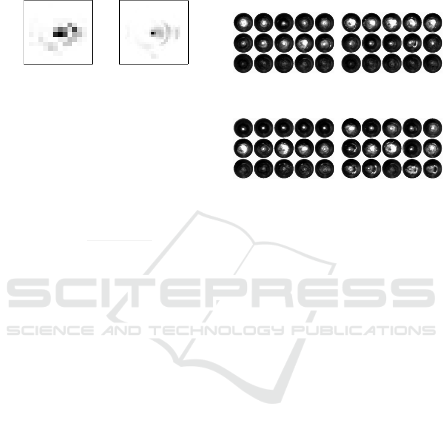
4.1 Results of Feature Ranking
Relevant features of the raw pixel intensities are
mostly located in the centre (see Fig. 6). This cor-
responds to the description in Sec. 2 where white re-
flections (regions) in the centre of the image indicate
good weldings. The ring structure, i.e. the neck of
the socket, can also be detected, which is relevant
for defective weldings (see Fig. 6 (left), Fig. 1 (lower
(a) sample std of white irreg-
ularity
(b) sample std of white aver-
aged clump area
(c) median of white extent
(d) entropy of white form-
factor
Figure 7: Example images with large values of the indicated
features (top row), medium (middle row) and small (bottom
row).
right)). Obviously, this depends neither on the size of
the images nor on their quantisation.
The most relevant features among the SGFs are:
• sample std. of white irregularity (see Fig. 7a),
• sample std. of white averaged clump area (see
Fig. 7b),
• mean of white displacements,
• mean of white irregularity, and
• mean of number of white components.
Not only the positions of white components are
important but also their size and irregularity. Com-
pared to the raw pixel intensities the SGFs can
also cover shape properties of local components (see
Fig. 6, 7a, 7b).
The most relevant SPECs are:
• median of the white extent (scaled by the number
of components (NOC), see Fig. 7c),
• median of the white compactness (scaled by
NOC),
• median of the white minimum distance from the
image centre (scaled by NOC),
• entropy of the white formfactor (scaled by NOC,
see Fig. 7d), and
• mean of white eccentricity (scaled by NOC).
Compared to the SGFs, more complex features be-
come significant, such as the extent or the form factor,
which can describe, for example, small white reflec-
tions in the image centre and holes in the socket of
defective cathodes simultaneously (seeFig. 7c, 7d).
WELDING INSPECTION USING NOVEL SPECULARITY FEATURES AND A ONE-CLASS SVM
151

Table 4: Frequency of the different local and global features
for the 48 most relevant features when combining SGFs and
SPECs.
name occurrence
scale by number of comp. 37
scale by relative area 11
white properties 48
black properties 0
local SPECs 47
local SGFs 1
global SPECs 22
global SGFs 16
When combining SGFs and SPECs only one SGF
is present in the 48 most relevant features which indi-
cates the quality of the SPECs (see Tab. 4). Further-
more, scaling by the number of components is more
important than scaling by their relative size. Hence,
small white regions are also responsible for defective
weldings, e.g. if they are located at the neck of the
socket (see Fig. 7(d) bottom row). Altogether, the
large number of extended shape properties (47) and
new global statistics (16) shows that the SPEC fea-
tures describe the relevant image properties of welded
cathodes more accurately than the SGFs.
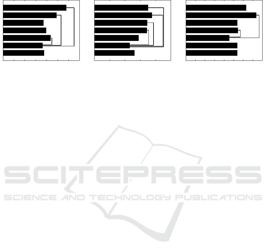
4.2 Results of Classification
The results for the different feature extraction meth-
ods applied to images of welded cathodes show sev-
eral aspects.
First, features of images of higher grey level depth
(6 – 8 bit) yield significantly lower error rates than
features of lower depth (see Fig. 9). This is inde-
pendent of the feature extraction method and confirms
the complexity of specular reflections in terms of grey
values.
Second, no significant difference between the two
image sizes could be observed, i.e. grey level reso-
lution is more important than spatial resolution (see
Fig. 9, 8). If the image size is lower than 12 ×12,
however, the higher relevance of the grey level depth
compared to image size does not hold, since the struc-
tures of the welded pin and the socket are merged,
e.g. holes and rings (see Fig. 3 bottom left) cannot
be detected. Also, SGFs and SPECs of images with
a higher grey value resolution perform significantly
better (see Fig. 9b, c).
Third, the SPECs (6 bit) have the lowest error
rate of 9.2% and perform significantly better than the
SGFs (7 bit, error rate 11.5%, p = 0.029, see Fig. 8).
Hence, SPECs describe the specular reflections of
SPEC (48 features)
SGF (48 features)
raw features 12×12 (144 fe atures)
raw features 24×24 (576 fe atures)
median of test errors
0 0.02 0.04 0.06 0.08 0.1 0.12 0.14 0.16 0.18
0.2
Figure 8: Comparison of the methods. Some of the signifi-
cant differences (p < 0.05) are indicated by black lines.
welded cathodes more precisely than SGFs and yield
a more accurate classification.
Fourth, the SPECs (6 bit) significantly outperform
the raw pixel intensities (error rate 18%, image depth
of 7 bit, see Fig. 8). Hence, the raw pixel intensi-
ties can only cover very simple image properties, e.g.
white reflections in the centre of the image, and they
are not able to describe holes or dependencies be-
tween reflections accurately.
5 CONCLUSIONS
We introduced a novel set of specularity features
(SPECs) for welding seam inspection and showed that
these features significantly outperform the statistical
geometric features as well as raw pixel intensities.
We extracted the relevant features of the SPECs and
found white regions in the centre of the image and
their shape to be of high importance for the classifi-
cation. The SPECs can cover several complex shape
properties and their dependencies and are, neverthe-
less, intuitive and computed efficiently. Hence, they
are well appropriate for the automatic inspection of
welding seams and can even be applied to a wider
range of machine vision problems concerning com-
plex specular reflections, such as surface inspection
or defect detection of specular objects.
The labelling of the datasets of solder joints or
other weldings is usually based on experts viewing
images and not on the actual functional test. Hence,
these labels are very subjective and do not necessar-
ily correspond to the physical and electrical properties
of the weldings. Therefore, additional information
about the welding, e.g. the conductivity, rigidity or
weld strength, has to be collected and combined with
a machine-vision based approach in order to improve
the results.
The results may further be improved using other
feature selection methods. However, the error rates
VISAPP 2009 - International Conference on Computer Vision Theory and Applications
152

(a) raw pixel intensities (12×12).
8bit
7bit
6bit
5bit
4bit
3bit
2bit
median of test errors
0 0.05 0.1 0.15 0.2 0.25 0.3
0.35
(b) SGFs.
8bit
7bit
6bit
5bit
4bit
3bit
2bit
median of test errors
0 0.05 0.1 0.15 0.2
0.25
(c) SPECs.
8bit
7bit
6bit
5bit
4bit
3bit
2bit
median of test errors
0 0.02 0.04 0.06 0.08 0.1 0.12 0.14
0.16
Figure 9: Medians of test errors. Black lines indicate a significant difference (p < 0.05) between two methods. Only significant
differences of the best depth level to all others are considered in the plot.
of the novel SPEC features are comparable to those
obtained by manual inspection.
REFERENCES
Boser, B., Guyon, I., and Vapnik, V. (1992). A training al-
gorithm for optimal margin classifiers. In Haussler,
D., editor, Proc. of the 5th Annual ACM Workshop
on Computational Learning Theory, pages 144–152.
ACM Press.
Chen, Y. Q., Nixon, M. S., and Thomas, D. W. (1995). Sta-
tistical geometrical features for texture classification.
Pattern Recognition, 28(4):537–552.
Chiu, S. and Perng, M. (2007). Reflection-area-based fea-
ture descriptor for solder joint inspection. Machine
Vision and Applications, 18(2):95–106.
Cortes, C. and Vapnik, V. (1995). Support-vector networks.
Machine Learning, 20(3):273–297.
Driels, M. and Lee, C. (1988). Feature selection for auto-
matic visual inspection of solder joints. The Int. Jour-
nal of Advanced Manufacturing Technology, 3:3–32.
Fukunaga, K. (1972). Introduction to Statistical Pattern
Recognition. Academic Press.
Kim, J. and Cho, H. (1995). Neural network-based inspec-
tion of solder joints using a circular illumination. Im-
age and Vision Computing, 13(6):479–490.
Ko, K. and Cho, H. (2000). Solder joints inspection using
a neural network and fuzzy rule-based classification
method. IEEE Transactions on Electronics Packaging
Manufacturing, 23(2):93–103.
Labusch, K., Timm, F., and Martinetz, T. (2008). Sim-
ple incremental one-class support vector classifica-
tion. In Rigoll, G., editor, Proc. of the 30th German
Pattern Recognition Symposium DAGM, volume 5096
of Lecture Notes in Computer Science, pages 21–30.
Springer.
Ong, T., Samad, Z., and Ratnam, M. (2008). Solder joint
inspection with multi-angle imaging and an artificial
neural network. The Int. Journal of Advanced Manu-
facturing Technology, 38(5–6):455–462.
Poechmueller, W., Glesner, M., Listl, L., and Mengel, P.
(1991). Automatic classification of solder joint im-
ages. In Proc. of the Int. Joint Conf. on Neural Net-
works, volume 2, pages 933–940. IEEE Computer So-
ciety Press.
Russ, J. C. (2007). The Image Processing Handbook. CRC
Press.
Sch
¨
olkopf, B., Platt, J. C., Shawe-Taylor, J., Smola, A. J.,
and Williamson, R. C. (2001). Estimating the support
of a high-dimensional distribution. Neural Computa-
tion, 13(7):1443–1471.
Stone, M. (1974). Cross-validatory choice and assessment
of statistical predictions. Journal of the Royal Statis-
tics Society, 36:111–147.
Tax, D. M. J. and Duin, R. P. W. (2004). Support vector data
description. Machine Learning, 54(1):45–66.
Timm, F., Klement, S., and Martinetz, T. (2008). Fast model
selection for maxminover-based training of support
vector machines. In Proc. of the 19th Int. Conf. on
Pattern Recognition, Florida, USA. IEEE Computer
Society Press. to appear.
Vapnik, V. (1995). The Nature of Statistical Learning The-
ory. Springer Verlag, New York.
Walker, R. and Jackway, P. T. (1996). Statistical geometric
features: Extensions for cytological texture analysis.
In Proc. of the 13th Int. Conf. on Pattern Recognition,
pages 790–794. IEEE Computer Society Press.
WELDING INSPECTION USING NOVEL SPECULARITY FEATURES AND A ONE-CLASS SVM
153