A DYNAMICAL MODEL FOR PULSATILE FLOW ESTIMATION IN
A LEFT VENTRICULAR ASSIST DEVICE
Abdul-Hakeem H. AlOmari, Andrey V. Savkin
School of Electrical Engineering and Telecommunications, The University of New South Wales, Sydney, Australia
Dean M. Karantonis
§
, Einly Lim
†
and Nigel H. Lovell
†
§
Ventracor Limited;
†
Graduate School of Biomedical Engineering, The University of New South Wales, Sydney, Australia
Keywords:
Implantable rotary blood pumps (iRBPs), Noninvasive pulsatile flow estimation, Left ventricular assist device
(LVAD).
Abstract:
In this paper, we propose a dynamical model for pulsatile flow estimation of an iRBP. Noninvasive measure-
ments of the motor power (VI) and pump impeller rotational speed (ω) were acquired from the pump controller
and used together with blood hematocrit (HCT) values as inputs to the model. A circulatory mock loop was
operated with different aqueous glycerol solutions, mimicking different values of viscosities equivalent to the
range of 20 - 50% of human blood HCT, to generate pulsatile flow data. Linear regression between estimated
pulsatile flow (Q
est
) and measured flow (Q
meas
) obtained from the mock loop resulted in a highly significant
correlation (R
2
= 0.957) and mean absolute error of e = 0.364 L/min. Also, R
2
= 0.902 and e = 0.317 L/min
were obtained when our model was validated using six sets of ex vivo porcine data. Furthermore, in steady
state, the solution of the presented model can be described by a previously designed and verified static model.
1 INTRODUCTION
The problem of noninvasive estimation of flow rate
has attracted the attention of many research groups
(for examples, see (Bertram, 2005)). It has been
shown that flow rate can be accurately estimated un-
der steady-state conditions (Malagutti et al., 2007;
Ayre et al., 2003; Funakubo et al., 2002; Kitamura
et al., 2000; Tsukiya et al., 2001).
Pulsatile flow estimation of iRBPs has been much
less frequently studied. This may be due to the large
number of factors that need to be taken into consid-
eration. Such factors may include the use of char-
acteristics curves of the pump where these are sensi-
tive to many physiological and mechanical parame-
ters like: changing blood viscosity, impeller inertia of
the pump.
In the present study, we used noninvasive feed-
back measurements of ω and VI to estimate the pul-
satile pump flowusing a newdynamicalmodel. When
operated in steady state conditions, our model can
provide an accurate estimate of the flow which agrees
with those obtained from the static model developed
in our laboratory under non-pulsatile conditions in
Malagutti et al. (2007). Another practically important
requirement for our dynamical model is its stability.
The proposed model will allow us to accurately study
and estimate the transient response and the dynamics
of the pulsatile flow.
2 MATERIALS AND METHODS
2.1 In vitro Pulsatile Experiments
A VentrAssist
T M
(Ventracor Limited, Sydney, Aus-
tralia) iRBP was connected in a circulatory mock loop
in a pulsatile environment. The loop was composed
of venous and arterial reservoir tanks, a silicone bag
which represented the left ventricle chamber (Karan-
tonis et al., 2007). Ventricular contraction was simu-
lated by periodically compressing the mock ventricle
with pneumatic pistons at a fixed rate. Arterial pres-
sure, central venous pressure, pump inlet and outlet
pressure were measured. Pulsatile flow was measured
by an Ultrasonic flow probe (Transonics Systems Inc.,
Ithaca, NY, USA). The instantaneous ω, motor volt-
402
H. AlOmari A., V. Savkin A., Karantonis D., Lovell N. and Lim E. (2009).
A DYNAMICAL MODEL FOR PULSATILE FLOW ESTIMATION IN A LEFT VENTRICULAR ASSIST DEVICE.
In Proceedings of the International Conference on Bio-inspired Systems and Signal Processing, pages 402-405
DOI: 10.5220/0001775604020405
Copyright
c
 SciTePress

age and current were accessed as feedback signals
from the controller. Speed was varied from 1800 to
3000 rpm in a stepwise increment of 100 rpm last-
ing for 30 s. For each step, systemic resistance was
also changed to cover the range of desired flows. The
sampling rate was 4 kHz for data recordings, but, in
further analysis, the data were down-sampled to 50
Hz.
2.2 Ex vivo Animals Experiments
The VentrAssist
T M
was acutely implanted in six
healthy pigs. In each pig, the inflow pump can-
nula was inserted into the apex of the left ventricle
while the outflow cannula was anastomosed to the as-
cending aorta (Karantonis et al., 2006). Indwelling
catheters (DwellCath, Tuta Labs, Lane Cove, NSW,
Australia) and pressure transducers (Datex-Ohmeda,
Homebush, NSW, Australia) were instrumented to the
pig’s native heart to measure left ventricle, left atrial,
aortic, and pump inlet pressures. Pump and aortic
flows were measured by ultrasonic flow probes from
the outlet cannula of the pump. Besides these sig-
nals, the noninvasive ω, motor current (I), and supply
voltage (V) were acquired from the pump controller.
The experimental data were sampled at 200 Hz. For
further information about data acquisition, see Karan-
tonis et al. (2006).
2.3 Dynamical Modeling
2.3.1 Static Flow Model
A noninvasive, steady-state average flow (Q
ss
) esti-
mator was designed in a non-pulsatile environment
for the iRBP. The estimator was based on VI, and ω.
The static equation for the flow estimator is based on
the work of Malagutti et al. (2007) and Ayre et al.
(2003) and is of the following form:
Q
ss
= a + bVI + cVI
2
+ dVI
3
+ eω+ pω
2
, (1)
where a, e, and p, are constants and the power coeffi-
cients b, c, and d were found to have a linear relation-
ship with the HCT (Malagutti et al., 2007).
2.3.2 Pulsatile Flow
In this section, we describe a dynamical model for
the iRBP. The main requirement for the dynamical
model is that any steady-state solution of the dynami-
cal model be a solution of the static equation (1). Fur-
thermore, we want any steady-state solution of the dy-
namical model to be stable. We introduce a variable
f(t) as follows:
f(t) = g(VI(t), ω(t)), (2)
where
g(VI(t), ω(t)) = a+ bVI(t) + cVI
2
(t) + dVI
3
(t)
+eω(t) + pω
2
(t). (3)
Here t = kh, h > 0 is the sampling interval, k =
0, 1, 2, 3, . . .. In other words, the variable f(t) repre-
sents the right-hand side of the static equation (1), de-
scribing the pump flow in steady-state. We introduce
a dynamical model of the form:
(A(∇) + B(∇))Q
est
(t) = B(∇) f(t), (4)
where Q
est
(t) is the output of the system which rep-
resents the estimated instantaneous values of the pul-
satile flow (Q(t)), f (t) is the input to the dynamical
system model, ∇ is the shift operator, A(∇), B(∇) are
polynomials defined as follows:
A(∇)Q
est
(t) =
n
∑
i=0
a
i
Q
est
(t − i+ 1), (5)
B(∇) f(t) =
m
∑
j=1
b
j
f(t − j+ 1). (6)
Here n is the model output order, and m is the model
input order satisfying the condition m ≤ n.
Now we describe all steady-state or constant so-
lutions of the equation (3). Let Q
est
(t) ≡ Q
0
and
f(t) ≡ f
0
for all t = 0, 1, 2. . ., then, we obtain from
(4) that
(A(1) + B(1))Q
0
= B(1) f
0
. (7)
We assume that A(1) = 0 and B(1) 6= 0. This yields
to the following conditions on parameters coefficients
of the model:
n
∑
i=0
a
i
= 0, (8)
m
∑
j=1
b
j
6= 0. (9)
Under the assumptions (8) and (9), it immediately fol-
lows from (7) that
Q
0
= f
0
. (10)
Since f(t) is defined by (2), (3), (10) it implies that
Q
0
is the corresponding solution of the equation (1).
Hence, steady-states of the dynamical model are de-
scribed by the static model.
Furthermore, if the system is stable i.e; all z :
A(z)+B(z) = 0 belong to | z |< 1 (all poles of the sys-
tem are inside the unit disk) (Ogata, 1995), then the
solution of the dynamical system (4) with any initial
conditions and with a constant input f
0
will converge
to the constant output Q
0
satisfying (10).
A DYNAMICAL MODEL FOR PULSATILE FLOW ESTIMATION IN A LEFT VENTRICULAR ASSIST DEVICE
403

2.3.3 Data Analysis
Data was divided into two sets, one set was used
for identification and training and the other to val-
idate the model. The off-line least squares method
(Ljung, 1999) was used to estimate the model coeffi-
cients. Values of parameter coefficients were chosen
so that the error between estimated Q
est
(t) and mea-
sured flow Q
meas
(t) was minimized. Also, parameters
should fulfill the assumptions defined in equations (8)
and (9). Mean absolute error (e), and correlation coef-
ficient (r) were used to check the performance of the
model as follows:
e =
1
N
N
∑
i=1
(Q
meas
(t) − Q
est
(t))
2
, (11)
r =
∑
N
i=1
(Q
meas
(t) − Q
meas
)(Q
est
(t) − Q
est
)
q
∑
N
i=1
(Q
meas
(t) − Q
meas
)
2
∑
N
i=1
(Q
est
(t) − Q
est
)
2
.
(12)
Here N is the length of data. Q
meas
, and Q
est
are the
mean values of the measured and estimated flows re-
spectively.
3 RESULTS
Least e and highest r between the estimated and mea-
sured flow in both mock loop and animal experiments
were obtained with system model orders of n = 3 and
m = 2.The resulting model is described as follows:
a
0
Q
est
(t) + (a
1
+ b
1
)Q
est
(t − 1) + (a
2
+ b
2
)Q
est
(t − 2)
+a
3
Q
est
(t − 3) = b
1
f(t − 1) + b
2
f(t − 2), (13)
where a
0
= 1, a
1
= −2.25, a
2
= 1.49, a
3
= −0.24,
b
1
= 0.27, b
2
= −0.25, Q
est
is the estimated pulsatile
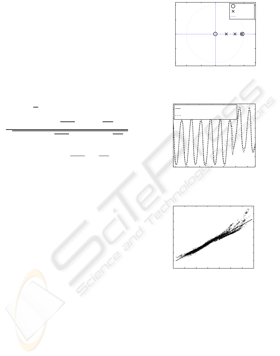
flow, and f(t) is the input signal. The poles-zeros plot
of the system shown in figure 1 demonstrates that the
model is stable. The dashed line in figure 2 shows part
of the estimated pulsatile and measured flow obtained
from the mock loop.
Linear regression analysis between Q
est
(t) and
Q
meas
(t) obtained from the mock loop experiments is
illustrated in figure 3. A highly significant correlation
between estimated and measured flow was obtained
with a small mean absolute error value.
During animal experimentation the values of HCT
were not measured. Instead, for each animal we
used the values of HCT that gave the best fit between
the estimated and measured flows in the steady state
model described in equation (1). Additionally, two
sets of data were removed from the analysis due to
−1 −0.5 0 0.5 1
−1
−0.5
0
0.5
1
Real Part
Imaginary Part
Zeros
Poles
Unit Disk
Figure 1: Poles-zeros plot of the system model described by
equation (13).
6094 6095 6096 6097 6098 6099 6100
4.5
5
5.5
6
6.5
7
7.5
Time (s)
Flow (L/min)
Measured Flow (Q
meas
)
Estimated Pulsatile Flow (Q
est
)
Figure 2: Estimated pulsatile flow compared with measured
flow obtained from mock loop.
−2 0 2 4 6 8 10 12
−2
0
2
4
6
8
10
12
14
Measured Flow (L/min)
Estimated Flow (L/min)
Q
est
= 1.080*Q
meas
+ 0.807
R
2
= 0.957
Figure 3: Linear regression plot between estimated versus
measured flow obtained from mock loop.
excessively noisy power signals. The comparison be-
tween estimated pulsatile and real flow for one of the
six animal experiments is shown in figure 4. Correla-
tion between estimated and real flows was highly sig-
nificant (R
2
= 0.902), with small mean absolute error
e = 0.317 L/min.
The response of the proposed model to abnor-
mal flow conditions associated with different pump-
ing states such as ventricular collapse (VC) and aortic
valve not opening (ANO) were accurately estimated
by the model (not shown).
BIOSIGNALS 2009 - International Conference on Bio-inspired Systems and Signal Processing
404

942 944 946 948 950
2
3
4
5
6
Time (s)
Flow (L)/min
Measured Flow (Q
real
)
Estimated Flow (Q
est
)
Figure 4: Estimated flow compared with measured one ob-
tained from pigs experiments.
4 DISCUSSION
In the present study, a dynamical model for pulsatile
flow estimation was successfully designed. In the pro-
posed model, the level of HCT was assumed to be
known. This is the major limitation of the presented
model.
Using an autoregressive with exogenous input
(ARX) model, Yoshizawa et al. (2002) developed a
pulsatile flow estimator (Yoshizawa et al., 2002). A
Mean absolute error of 1.66 L/min, and a correlation
coefficient of 0.85 were obtained when another ARX
model has used to compensate for HCT. Tsukiya et
al. (2001) showed that the non-pulsatile flow rate es-
timator was able to monitor the instantaneous flow
(Tsukiya et al., 2001). To compare, our proposed
model resulted in a high correlation coefficient R
2
=
0.957 with e= 0.364 L/min in mock loop. Also R
2
=
0.902 and e= 0.317 L/min were obtained using ex vivo
animals data.
Ayre et al. (2003) were successfully estimated
an average flow for non-pulsatile and pulsatile flow
(Ayre et al., 2003). More recently, pulsatile flow was
accurately estimated by Karantonis et al. (2007). Al-
though these studies produced acceptable results, they
did not study the stability of the transient response of
the pump flow which is one of the outcomes of the
present study.
5 CONCLUSIONS
A dynamical model for an iRBP has been presented
and shown to accurately estimate the pulsatile flow
using noninvasive measurements of power and speed.
Furthermore, the proposed model is stable and its set
of steady states is identical to the set of solutions of
the previously derived static model.
ACKNOWLEDGEMENTS
This work was supported by The Australian Research
Council.
REFERENCES
Ayre, P. J., Lovell, N. H., and Woodard, J. C. (2003).
Non-invasive flow estimation in an implantable rotary
blood pump: a study considering non-pulsatile and
pulsatile flow. Physiol Meas, 24:179–89.
Bertram, C. (2005). Measurement for implantable rotary
blood pumps. Physiol Meas, 26:R99–R117.
Funakubo, A., Ahmed, S., Sakuma, I., and Fukui, Y. (2002).
Flow rate and pressure head estimation in a centrifugal
blood pump. Artif Organs, 26:985–90.
Karantonis, D. M., Cloherty, S. L., Mason, D. G., Ayre, P. J.,
and Lovell, N. H. (2007). Noninvasive pulsatile flow
estimation for an implantable rotary blood pump. In
Proceedings of the 29th Annual International Confer-
ence of the IEEE EMBS.
Karantonis, D. M., Lovell, N. H., Ayre, P. J., Mason, D. G.,
and Cloherty, S. L. (2006). Identification and classi-
fication of physiologically significant pumping states
in an implantable rotary blood pump. Artif Organs,
30:671–9.
Kitamura, T., Matsushima, Y., Kono, S., Nishimura, K.,
Komeda, M., Yanai, M., Kijima, T., and Nojiri, C.
(2000). Physical model-based indirect measurements
of blood pressure and flow using a centrifugal pump.
Artif Organs, 24:589–93.
Ljung, L. (1999). System Identification: Theory for the
user. Prentice Hall PTR, USA, 2nd edition.
Malagutti, N., Karantonis, D.M., Cloherty, S. L., Ayre, P. J.,
Mason, D. G., Salamonsen, R. F., and Lovell, N. H.
(2007). Noninvasive average flow estimation for an
implantable rotary blood pump: a new algorithm in-
corporating the role of blood viscosity. Artif Organs,
31:45–52.
Ogata, K. (1995). Discrete-Time Control Systems. Prentice
Hall Inc., USA, 2nd edition.
Tsukiya, T., Taenaka, Y., Nishinaka, T., Oshikawa, M.,
Ohnishi, H., Tatsumi, E., Takano, H., Konishi, Y., Ito,
K., and Shimada, M. (2001). Application of indirect
flow rate measurement using motor driving signals to
a centrifugal blood pump with an integratedmotor. Ar-
tif Organs, 25:692–96.
Yoshizawa, M., Sato, T., Tanaka, A., Abe, K., Takeda, H.,
Yambe, T., Nitta, S., and Nose, Y. (2002). Sensor-
less estimation of pressure head and flow of a con-
tinuous flow artificial heart based on input power and
rotational speed. ASAIO Journal, 48:443–48.
A DYNAMICAL MODEL FOR PULSATILE FLOW ESTIMATION IN A LEFT VENTRICULAR ASSIST DEVICE
405