WEAKENED WATERSHED ASSEMBLY FOR REMOTE SENSING
IMAGE SEGMENTATION AND CHANGE DETECTION
Olivier Debeir
1
, Hussein Atoui
2
1
L.I.S.A.,
2
M.L.G., Universit´e Libre de Bruxelles, 50 av.F.D.Roosevelt CP165/57, 1050 Brussels, Belgium
Christophe Simler
Royal Military Academy, Brussels, 50 av.F.D.Roosevelt 1050 Brussels, Belgium
Nadine Warz´ee
3
, El´eonore Wolff
4
3
L.I.S.A.,
4
I.G.E.A.T., Universit´e Libre de Bruxelles, 50 av.F.D.Roosevelt 1050 Brussels, Belgium
Keywords:
Segmentation, Watershed, Multiclassifier system, Remote sensing.
Abstract:
Marked watershed transform can be seen as a classification in which connected pixels are grouped into com-
ponents included into the marks catchment basins.The weakened classifier assembly paradigm has shown its
ability to give better results than its best member, while generalization and robustness to the noise present in
the dataset is increased. We promote in this paper the use of the weakened watershed assembly for remote
sensed image segmentation followed by a consensus (vote) of the segmentation results. This approach allows
to, but is not restricted to, introduce previously existing borders (e.g. for the map update) in order to constraint
the segmentation. We show how the method parameters influence the resulting segmentation and what are the
choices the practitioner can make with respect to his problem. A validation of the obtained segmentation is
done by comparing with a manual segmentation of the image.
1 INTRODUCTION
Region classification is becoming increasingly more
used in the remote sensing applications as reviewed
in (Carleer et al., 2005). The watershed transform
is known to give an interesting solution for image
segmentation by creating closed contours (Beucher
and Lantuejoul, 1979). Watershed transform has
been widely used in remote sensing image segmen-
tation, its major benefits being an extreme sensitiv-
ity to detect borders and the outcome of closed con-
tours which are useful for consecutive segmentation
exploitation (Chen et al., 2004). Due to its extreme
sensitivity, the use of the watershed transform may
lead to the creation of many unwanted local water-
shed basins in a highly textured area. This prob-
lem increases dramatically with the image resolution
available. Over-segmentation issue is usually tackled
by three, possibly complementary, ways: (i.) image
low pass or similar pre-filtering that eliminates lo-
cal minima and therefore diminishes the number of
unwanted watershed basins, (ii.) using the marked
watershed transform to limit the basins to only those
which are marked and (iii.) by using a basin fusion
step after the watershed transform. This step often
integrates multi-spectral data that are available. As
described by (Noyel et al., 2007), not all the borders
present in the image are of interest. Indeed noise or
very small structures cause local minima (in the gra-
dient image) that give rise to small regions (i.e. over-
segmentation). On the contrary, some borders are
important and significant with respect to the tackled
problem and exhibit more stability (e.g. to marker
selection). Randomization of such learning can be
done by modifying the marks (Noyel et al., 2007),
but, similarily to the weak classifier paradigm, one
can also influence the result of the watershed trans-
form by modifying the data (i.e. the gradient image)
itself. Recent developments have shown that water-
shed transform randomized by mean of random marks
gives interesting results both in unsupervised (Noyel
et al., 2007; Angulo and Jeulin, 2007) and supervised
approach (Debeir et al., 2008). The way to limit the
number of watershed basins is here linked to there sta-
bility to perturbations, only stable/robust borders are
kept. A similar result can be obtained by introducing
129
Debeir O., Atoui H., Simler C., Warzée N. and Wolff E. (2009).
WEAKENED WATERSHED ASSEMBLY FOR REMOTE SENSING IMAGE SEGMENTATION AND CHANGE DETECTION.
In Proceedings of the Fourth International Conference on Computer Vision Theory and Applications, pages 129-134
DOI: 10.5220/0001755501290134
Copyright
c
 SciTePress

noise inside the gradient image itself (Debeir et al.,
2008). We will show here that a combination of ran-
dom marks and gradient perturbation allows to tackle
efficiently remote sensing image segmentation as pre-
processing step to region classification. Moreover the
proposed method allows to include a pre-existing bor-
der map in order to constrain the segmentation pro-
cess as expected for the map update framework.
2 MATERIAL
The study area is situated in the southeast of Belgium,
near the city of Arlon. The image data are panchro-
matic QuickBird images acquired in 1999 and 2004
with a resolution of 0.6 m. Borders of the panchro-
matic 2004 image are computed by a classical mor-
phological filter of radius 1 (4 neighbors). The opera-
tion is achieved on the complete 11 bit panchromatic
image dynamic. The obtained gradient is converted
into 8 bit image (levels higher or equal to 255 are set
to 255). Both images of 1999 and 2004 where man-
ually segmented. Borders of 1999 labels are consid-
ered as a priori knowledge, indeed in the context of
map update, the pre-existing map can be considered
as known and serves as input to the image segmenta-
tion. The labels of 2004 will be used exclusively as
validation and are not used during the segmentation.
All images are considered as registered with respect
to the smallest available detail. Label images are ras-
terized from the supervised label images of year 1999
and 2004. In order to put the borders between the
labels, the image is oversampled two times in both
dimensions. Other raster images are extended within
the same proportions (nearest value).
3 METHOD
Numerous theoretical and experimental studies show
that a combination of several diverging classifiers
(also called multiple classifier system or ensemble ap-
proach) is an effective technique for reducing predic-
tion errors (Kittler et al., 1998; Bay, 1998; Breiman,
1996). The key of this improvement relies greatly
on the degree of decorrelation of the errors between
the classifiers. One approach to create error diversity
is to perturb input data in order to train the compo-
nent classifiers with different training sets (weakened
classifiers). We promote here the use of image per-
turbation and marker randomization in order to build
the assembly of randomized segmentation based on
marked watershed transform.
(a.)
Label
1999
Panchro
2004
gradient
label
border
1999
border
counters
random
marks
Marked
Watershed
Transform
perturbated
gradient
Watershed
borders
+
priors
random
marks
Marked
Watershed
Transform
perturbated
gradient
Watershed
borders
+
priors
random
marks
Marked
Watershed
Transform
perturbated
gradient
Watershed
borders
+
+
1...NITER
(optional)
(b.)
Label
2004
border
counters
counters
thresholded
watershed
transform
segmented
image
region
label
border
label
border
2004
borders
keeping stronger watershed borders
closing borders
Validation
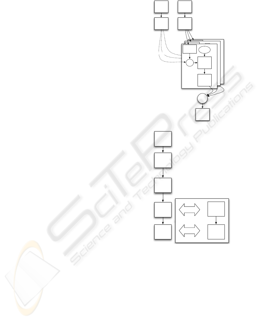
Figure 1: Ensemble approach: (a.) the counter image is
generated by the assembly of randomized watershed trans-
form (perturbated gradient and randomized marks), (b.) the
obtained borders are compared with the supervision.
Figure 1 illustrates the overall segmentation pro-
cess with (a.) the randomization phase and (b.) the
consensus phase. The different steps are explained in
the following paragraphs
3.1 Image Perturbation
A random slope (SLOPE) image based on random
Fourier transform image is added to the gradient im-
age of 2004 (the SLOPE is scaled to an interval
of [−MAXSLOPE,+MAXSLOPE]). As result, some
VISAPP 2009 - International Conference on Computer Vision Theory and Applications
130

weak gradient levels present in the original image
can be reinforced, whereas others are smoothened.
SLOPE image is generated by applying the inverse
Fourier transform to a randomly generated frequency
domain image. Let f be an empty image (imaginary)
of size equal to the gradient image (image origin is
centered). We add n pixels (here we arbitrarily used
n = 5) of value 1+j for randomly generated positions
as follows:
f(x,y) =

1+ j ∀(x
k
,y
k
) = (ρ
k
cos(θ
k
),ρ
k
sin(θ
k
))
0 else
(1)
where
θ
k
= 2πU(0, 1)
ρ
k
= 1 + f
max
U(0,1)
k = 1· · · n
(2)
The f
max
parameters limits the upper bound of the
spatial frequency injected in the SLOPE. It was set
experimentaly to 10. The SLOPE image is normal-
ized in [0,1] using:
SLOPE = (F
−1
( f))/ max(F
−1
( f)) (3)
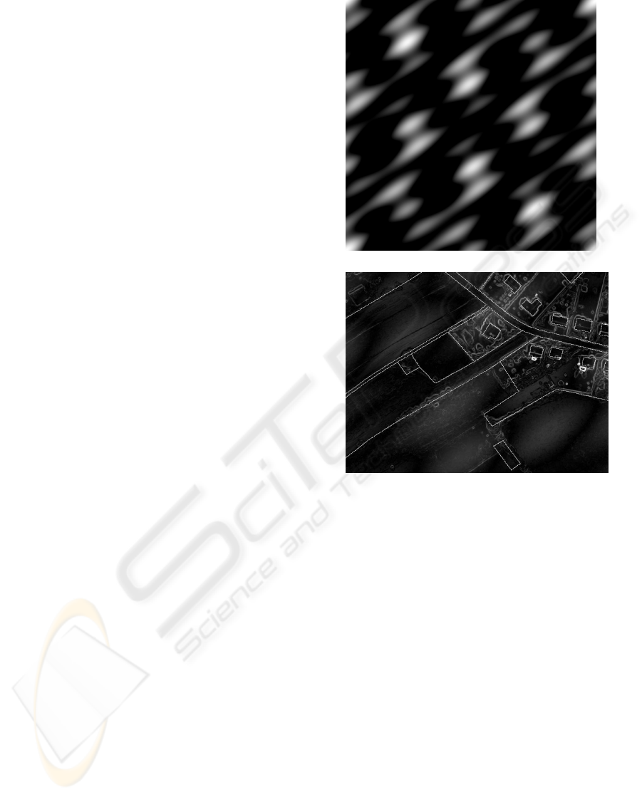
Figure 2 (a.) shows an example of a random
SLOPE obtained. Due to the nature of the tack-
led problem (map update), one might be interested
in adding existing borders to the segmentation (e.g.
from an old labelized image of the same region). It
is indeed common for an updated image to retrieve
many borders from a previously remote sensed im-
age. Of course some borders may also disappear, this
case will be discussed further.
In order to inject this a priori knowledge, the ex-
isting borders of the 1999 label image are injected af-
ter the gradient perturbation. Each pixel of the 1999
image belonging to a label border is forced to the
maximal gradient value (255). An example of a mod-
ified gradient image is illustrated in figure 2(b.).
3.2 Randomized Marked Watershed
Marker image is built by randomly (using a uniform
distribution) marking pixels inside the image domain.
The parameter DENSITY gives the number of marks
generated per image pixel.
3.3 Watershed Assembly Consensus
NITER iterations of the modified gradient image and
random marks are built. For each iteration, marked
watershed transform is applied on the modified gradi-
ent image using random marks (one different gradient
perturbation is computed for each iteration). This re-
sults in one segmentation as illustrated in figure 1(a.).
The watershed basins borders obtained by each seg-
mentation are accumulated into a COUNTER image.
(a.)
(b.)
Figure 2: Gradient perturbation: (a.) random slope obtained
by inverse Fourier transform (SLOPE) and (b.) SLOPE
added to the 2004 gradient image (detail) with a priori
(1999) borders in overlay.
The COUNTER image has high values for pixels fre-
quently selected as watershed borders (i.e. robust bor-
ders), while low COUNTER values are pixels rarely
involved in label separation. COUNTER pixels hav-
ing a value greater than a selected thresholdCOUNT
th
value keep most robust border. In order to close the
obtained borders, the watershed transform is applied
to the thresholded COUNTER image as illustrated in
1(b.).
3.4 Segmentation Result Comparison
Region classification results depend greatly on the
quality of the region used. We can identify two main
defects for the segmentation: (i.) over-segmentation
and (ii.) under-segmentation. If region borders
overlap objects belonging to different classes (under-
segmentation error), the classification process will
perform poorly. On the contrary, if segmenta-
WEAKENED WATERSHED ASSEMBLY FOR REMOTE SENSING IMAGE SEGMENTATION AND CHANGE
DETECTION
131

tion splits labels into numerous sub-regions (over-
segmentation) one loses the benefit of using region
rather than using pixels for the classification process.
In order to assess the quality of obtained segmenta-
tion, we compare it with the manually obtained bor-
ders of the same image. We implement different
image partition comparison coefficients described in
the literature (Unnikrishnan and Hebert, 2005; Jiang
et al., 2006). In (Unnikrishnan and Hebert, 2005),
authors compare different kinds of methods (metrics)
with respect to the application (e.g. same number of
labels or not). If label images are C1 and C2, one de-
fines the Normalized Mutual Information (NMI) as:
NMI(C
1
,C
2
) =
∑
c
i
∈C
1
∑
c
j
∈C
2
p(c
i
,c
j
)log
p(c
i
,c
j
)
p(c
i
)p(c
j
)
(4)
where p(c
i
,c
j
) is the frequence of observing one
pixel belonging to label i in C1 and to label j in C2
normalized by the total number of pixel in the im-
age. Because changes are very subtle between the two
available datasets (1999 and 2004) we extract an other
measure more focused on label borders differences.
Border changes are counted as ADD
rel
(C
1
,C
2
) pixels
borders (i.e. border present in C2 that is not a border
in C1) and REM
rel
(C
1
,C
2
) (i.e. border present in C1
that is not a border in C2) normalized by the number
of image pixels.
4 APPLICATION
The map update framework can be stated as follows:
we have a database containing the vectorial descrip-
tion of objects of interest at a certain moment (labels
from 1999 represented in figure 3(a.)). A new im-
age is acquired (e.g. by remote sensing) and regis-
tered to the database (the background image of the
figure 3 (c.) and (d.) is the 2004 panchromatic im-
age). The map update consists in creating a new label
image (vectors) for the acquired image eventually us-
ing existing labels as support.
The randomized watershed assembly has been ap-
plied to the 2004 image and segmentation results
were compared to the manual segmentation. Figure
3 shows an example of resulting segmentation.
In the given example, objects appear (+ sign), oth-
ers disappear (- sign). The colors in figure 3 are used
as follows : in (c.) the color overlay corresponds to
the label (i.e. pre-existing) of year 1999 (i.e. same
as (a.)), this corresponds to the a priori knowlege. In
(d.) the color overlay corresponds to the 2004 label
(i.e. same as (b.)) which is the updated version of
1999 label.
+
+
-
1
3
7
5
4
6
2
(d.)
(c.)
(b.)
(a.)
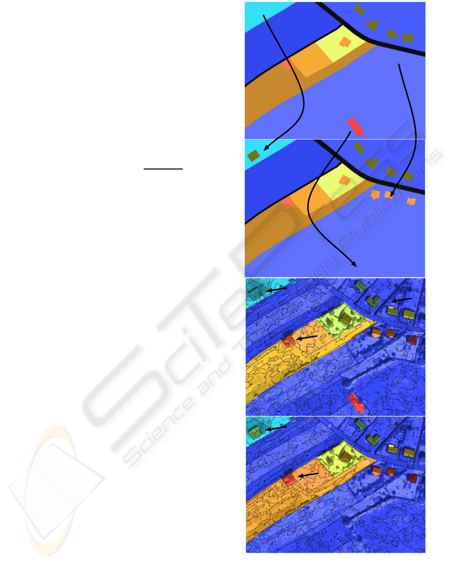
Figure 3: Segmentation results (detail): (a.) labels of 1999,
(b.) labels of 2004, (c.) segmentation not using a priori
knowledge (color overlay from the 1999 labels) and (d.)
segmentation using a priori knowledge, i.e. borders of the
1999 labels (color overlay from the 2004 labels).
VISAPP 2009 - International Conference on Computer Vision Theory and Applications
132

In the image (c.) the segmentation was done without
using the a priori knowledge, one can see that water-
shed basins follow approximately the labels borders.
Using a priori knowlege (image (d.)) enhances the
quality of these borders by forcing pre-existing bor-
ders (e.g. (3) and (4) in figure 3). Of course a label
present in 1999 and not present in 2004 will create in-
correct borders as illustrated by (5) and (6) in figure
3. For both approaches (with and without a priori)
the method is able to segment thin structures (e.g. as
illustrated by (7) in figure 3(c.)). New structures are
well detected (e.g. (1) and (2) in figure 3 with and
without using a priori knowledge. Man made struc-
tures such as houses and roads are well segmented
(a small over-segmentation occurs on different roof
slopes). Globally, all the objects are well detected in
the sense that all object borders are included inside
the segmentation for both methods using or not using
a priori knowledge (pre-existing borders). Most la-
belized objects are over-segmented, as illustrated by
(2) in figure 3 , this is mainly due to the existing con-
trast (robust borders) inside objects of interest. Over-
segmentation, if limited, would be addressed in a fur-
ther classification scheme not illustrated here. The
injection of a priori knowledge is well illustrated in
figure 3 (d.), borders of object (4) are found by the
segmentation procedure while randomized watershed
assembly without using priors gives more irregular
borders (object (3)). In the case of object that dis-
appears from one image to the other (as illustrated by
(6) where an object present in the database is missing
in the new image), injection of a priori knowledge
may generate false borders. This problem is also con-
sidered as over-segmentation and will be tackled in
further classification steps.
5 PARAMETERS SETTINGS
As often the presented segmentation method relies on
several parameters. Practitioner likes to have some
rule of the thumb to have at least a starting point for
the parameters setting. The method we propose re-
quires the settings of basically four parameters : (i.)
the marker density function (DENSITY), (ii.) the ran-
dom slope (MAXSLOPE), (iii.) the number of voters
(NITER) and (iv.) the threshold of the counter value
(COUNT
th
). We tested the variations observed on the
results for a typical range for each of these parameters
and summarized the results below.
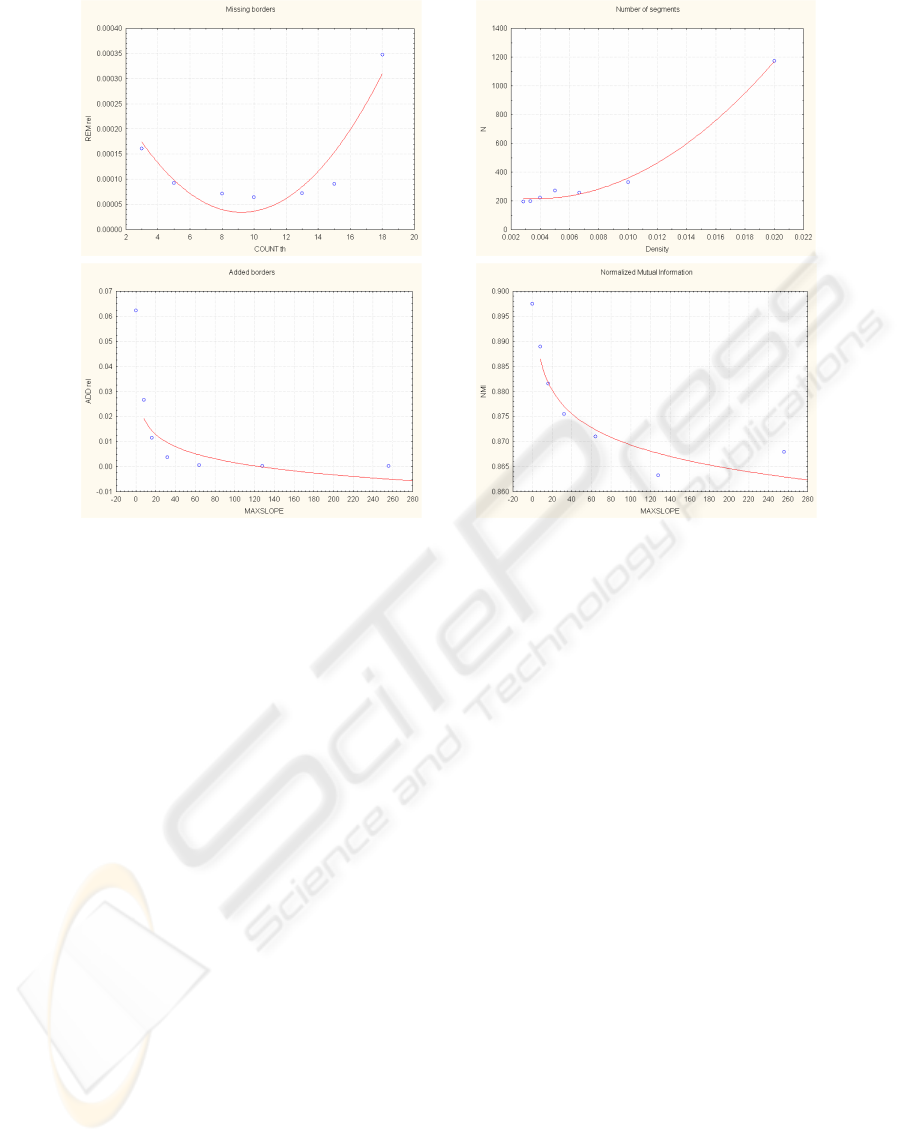
Figure 4 (a.) shows how relative missed border
evolves with respect to COUNT
th
. The curve exhibits
a minimum value around 10 on a total number of iter-
ations equal to 35 which means that a border is to be
considered robust if its occurrence is higher that 1/3
of the total number of iterations. DENSITY of the
random markers influences positively the number of
segments as illustrated in figure 4 (b.) which is con-
sistent with the marked watershed properties. Con-
cerning the MAXSLOPE parameter, it is negatively
linked with the number of ADD
rel
borders (figure 4
(c.)), as well as with the number of segments (data not
shown). This is coherent with the fact that small local
gradient can be randomly smoothed by the SLOPE
perturbation. TheCOUNT
th
parameter tunes the level
of over-segmentation, it can be easily set interactively
by the user to select the segmentation granularity.
6 CONCLUSIONS
We propose the use of a weakened assembly of
marked watershed transform for segmenting remote
sensed imagery. This technique relies on the pertur-
bation of the gradient image on one hand and on a
random marking on the other hand. This approach
also allows to take previsouly detected borders into
account, which is useful when applied to map up-
date. Different method parameters are identified and
characterized with respect to the quality of the seg-
mentation. Watershed randomization allows to detect
small (thin) objects but also allows to limit the ob-
tained segments only to the stable ones (i.e. limiting
the over-segmentation). In comparison to manual la-
belling, the proposed method still gives more labels.
However the obtained borders are consistent with the
supervision, meaning that expected labels are well de-
tected, but composed of few sub-labels. We show
that under-segmentation is kept low by evaluating the
missed borders. In this work, we do not use any spec-
tral or contextualinformation. This will be considered
in further automatic classification process.
ACKNOWLEDGEMENTS
The authors want to thank IGN Belgium for giving
access to the TOP10V-GIS database, the DGA for the
remote sensed image, and F. De Groef for the proof-
ing. The image data were funded by the European
Commission and made available by the JRC IPSC
GeoCAP unit through the Ministry of Agriculture
(Walloon Region, Belgium). Debeir O., Simler C.
and Atoui H. are granted by IRSIB-IWOIB Institute
for the encouragement of Scientific Research and
Innovation of Brussels. The authors want to thank the
reviewers for there constructive remarks.
WEAKENED WATERSHED ASSEMBLY FOR REMOTE SENSING IMAGE SEGMENTATION AND CHANGE
DETECTION
133

(a.) (b.)
(c.) (d.)
Figure 4: Method parameters influence: (a.) REM
rel
(C
1
,C
2
) vs COUNT
th
, (b.) number of segment vs marker DENSITY, (c.)
ADD
rel
(C
1
,C
2
) vs MAXSLOPE and (d.) NMI vs MAXSLOPE.
REFERENCES
Angulo, J. and Jeulin, D. (2007). Stochastic watershed seg-
mentation. In Banon, G. J. F., Barrera, J., Braga-Neto,
U. d. M., and Hirata, N. S. T., editors, Proceedings,
volume 1, pages 265–276, S˜ao Jos´e dos Campos. Uni-
versidade de S˜ao Paulo (USP), Instituto Nacional de
Pesquisas Espaciais (INPE).
Bay, S. (1998). Combining nearest neighbor classifiers
through multiple feature subsets. In Proc. 15th In-
ternational Conf. on Machine Learning, pages 37–45.
Morgan Kaufmann, San Francisco, CA.
Beucher, S. and Lantuejoul, C. (1979). Use of watersheds
in contour detection. In International Workshop on
Image Processing: Real-time Edge and Motion De-
tection/Estimation, Rennes, France.
Breiman, L. (1996). Bagging predictors. Machine Learn-
ing, 24(2):123–140.
Carleer, A., Debeir, O., and Wolff, E. (2005). Assessment
of very high spatial resolution satellite image segmen-
tations. Photogrammetric Engineering and Remote
Sensing, 71(11):1285–1294.
Chen, Q., Zhou, C., Luo, J., and Ming, D. (2004). Fast
segmentation of high-resolution satellite images us-
ing watershed transform combined with an efficient
region merging approach. In IWCIA, pages 621–630.
Debeir, O., Adanja, I., Warze, N., Ham, P. V., and De-
caestecker, C. (2008). Phase contrast image segmenta-
tion by weak watershed transform assembly. In ISBI,
pages 724–727. IEEE.
Jiang, X., Marti, C., Irniger, C., and Bunke, H. (2006).
Distance measures for image segmentation evaluation.
EURASIP J. Appl. Signal Process., (1):209.
Kittler, J., Hatef, M., Duin, R. P. W., and Matas, J. (1998).
On combining classifiers. IEEE Trans Pattern Analy-
sis and Machine Intelligence, 20(3):226–239.
Noyel, G., Angulo, J., and Jeulin, D.(2007). Random germs
and stochastic watershed for unsupervised multispec-
tral image segmentation. In KES (3), pages 17–24.
Unnikrishnan, R. and Hebert, M. (2005). Measures of
similarity. In Application of Computer Vision, 2005.
WACV/MOTIONS ’05 Volume 1. Seventh IEEE Work-
shops on, volume 1, page 394.
VISAPP 2009 - International Conference on Computer Vision Theory and Applications
134