USING EXPANDED MARKOV PROCESS AND JOINT

DISTRIBUTION FEATURES FOR JPEG STEGANALYSIS

Qingzhong Liu

1,2

, Andrew H. Sung

1,2

, Mengyu Qiao

Depart of Computer Science,

Institute for Complex Additive Systems Analysis

New Mexico Tech, Socorro, NM 87801, U.S.A.

Bernardete M. Ribeiro

Department of Informatics Engineering, University of Coimbra, Coimbra, Portugal

Keywords: Steganalysis, JPEG, Image, SVM, Markov, Pattern recognition.

Abstract: In this paper, we propose a scheme for detecting the information-hiding in multi-class JPEG images by

combining expanded Markov process and joint distribution features. First, the features of the condition and

joint distributions in the transform domains are extracted (including the Discrete Cosine Transform or DCT,

the Discrete Wavelet Transform or DWT); next, the same features from the calibrated version of the testing

images are extracted. A Support Vector Machine (SVM) is applied to the differences of the features

extracted from the testing image and from the calibrated version. Experimental results show that this

approach delivers good performance in identifying several hiding systems in JPEG images.

1 INTRODUCTION

To enable covert communication, steganaography is

the technique of hiding data in a digital media.

Digital image is currently one of the most popular

digital media for carrying covert messages. The

innocent image is called carrier or cover; and the

adulterated image carrying some hidden data is

called stego-image or steganogram. In image

steganography, the common information-hiding

techniques implement information-hiding by

modifying the pixel values in space domain or

modifying the coefficients in transform domain.

Some other information hiding techniques include

spread spectrum steganography (Marvel et al.,

1999), statistical steganography, distortion, and

cover generation steganography (Katzenbeisser and

Petitcolas, 2000), etc.

The objective of steganalysis is to discover the

presence of hidden data. To this date, some

steganographic embedding methods such as LSB

embedding, spread spectrum steganography, and

LSB matching, etc. (Fridrich et al., 2002), (Harmsen

and Pearlman, 2004), (Harmsen and Pearlman,

2003), (Ker, 2005), (Liu and Sung, 2007), (Liu et al.,

2006; Liu et al., 2008a, 2008b) have been success-

fully steganalyzed.

JPEG image is one of the most popular media on

the Internet and easily used to carry hidden data;

many information-hiding methods and/or tools on

the Internet implement hiding message in JPEG

images, therefore, it’s important for many purposes

to design a reliable algorithm to decide whether a

JPEG image found on the Internet carries hidden

data or not. There are a few methods for detecting

JPEG steganography. One of them is Histogram

Characteristic Function Center Of Mass (HCFCOM)

for detecting noise-adding steganography (Harmsen

and Pearlman, 2003) another well-known method is

to construct the high-order moment statistical model

in the multi-scale decomposition using wavelet-like

transform and then apply learning classifier to the

high order feature set (

Lyu and Farid, 2005). Fridrich

et al. presented a method to estimate the cover-

image histogram from the stego-image (Fridrich et

al., 2002). Another new feature-based steganalytic

method for JPEG images was proposed where the

features are calculated as an L1 norm of the

difference between a specific macroscopic

functional calculated from the stego-image and the

same functional obtained from a decompressed,

cropped, and recompressed stego-image (Fridrich,

226

Liu Q., H. Sung A., Qiao M. and Ribeiro B. (2009).

USING EXPANDED MARKOV PROCESS AND JOINT DISTRIBUTION FEATURES FOR JPEG STEGANALYSIS.

In Proceedings of the International Conference on Agents and Artiﬁcial Intelligence, pages 226-231

DOI: 10.5220/0001658402260231

 SciTePress

2004). Harmsen and Pearlman implemented a

detection scheme using only the indices of the

quantized DCT coefficients in JPEG images

(Harmsen and Pearlman, 2004). Recently, Shi et al.

proposed a Markov process based approach to

effectively attacking JPEG steganography, which

have remarkably better performance than general

purpose feature sets (Shi et al., 2007). By applying

calibration to Markov features, Pevny and Fridrich

merged their DCT features and calibrated Markov

features to improve the steganalyis performance in

JPEG images (Pevny and Fridrich, 2007).

Based on the Markov process based approach

(Shi et al., 2007) and the calibration version (Pevny

and Fridrich, 2007), in this article, we expand the

Markov features to inter-blocks of the DCT domain

and to the wavelet domain, and design the features

of the joint distribution on the DCT domain and the

wavelet domain, and calculate the difference

between the features from the testing images and the

same features from the calibrated ones. We

successfully improve the detection performance in

multi-class JPEG images.

The rest of this article is organized as follows:

the second section expands the Markov features; the

third presents the features of joint distribution of the

transform domains; the forth explains the calculation

of the calibrated version of the images and the

feature extraction; the fifth introduces experiments

and compares the detection performances of the

different feature sets; and followed by our

conclusions in the sixth.

2 EXPANING MARKOV

PROCESS

2.1 Introduction to Markov Approach

Shi et al. proposed the Markov process by modeling

the differences between absolute values of

neighboring DCT coefficients as a Markov process

(Shi et al., 2007). The matrix F (u, v) stands for the

absolute values of DCT coefficients of the image.

The DCT coefficients in F (u, v) are arranged in the

same way as pixels in the image by replacing each 8

× 8 block of pixels with the corresponding block of

DCT coefficients. Four difference arrays are

calculated along four directions: horizontal, vertical,

diagonal, and minor diagonal, denoted F

(u, v), F

(u, v), and F

(u, v), respectively.

(,) (,) ( 1,)

uv Fuv Fu v=−+

(1)

(,) (,) (, 1)

Fuv Fuv Fuv

−+

(2)

(,) (,) ( 1, 1)

Fuv Fuv Fu v

−++

(3)

(,) ( 1,) (, 1)

Fuv Fu v Fuv

+− +

(4)

Here we just utilize F

(u, v) and F

(u, v). The

four transition probability matrices M1

, M1

, and M1

are set up as

((,) ,( 1,) )

1(,)

((,) )

uv iF u v j

Mij

Fuv i

−

=+=

∑∑

(5)

((,) ,(, 1) )

1(,)

((,) )

Fuv iFuv j

Mij

Fuv i

−−

=+=

∑∑

(6)

((,) ,( 1,) )

1(,)

((,) )

uv iF u v j

Mij

Fuv i

−−

=+=

∑∑

(7)

((,) ,(, 1) )

1(,)

((,) )

Fuv iFuv j

Mij

Fuv i

−

=+=

∑∑

(8)

Where

and

denote the dimensions of the

image and

= 1 if and only if its arguments are

satisfied. Due to the range of differences between

absolute values of neighboring DCT coefficients

could be quite large, the range of i and j is limited [-

4, +4]. Thus, all Markov features consist of 4 × 81 =

324 features.

2.2 Expanding Markov Process

From our standpoint, the original Markov features

utilize the relation of neighboring DCT coefficients

in the intra-DCT-block. Actually, the neighboring

DCT coefficients on the inter-block have the similar

relations; we expand the original Markov features to

the neighboring DCT coefficients on the inter-

blocks.

2.2.1 Inter-DCT block Markov Process

In addition to the transition matrices constructed on

the intra-difference, we also construct the transition

matrices based on the inter-DCT blocks.

First, the horizontal and vertical difference arrays

on the inter-block are defined as follows:

(,) (,) ( 8,)

uv Fuv Fu v

−+

(9)

(,) (,) (, 8)

Duv Fuv Fuv

−+

(10)

The four transition probability matrices M2

, M2

and M2

are constructed as follows.

USING EXPANDED MARKOV PROCESS AND JOINT DISTRIBUTION FEATURES FOR JPEG STEGANALYSIS

227

((,),( 8,) )

2(,)

((,))

uv iD u v j

Mij

Duv i

−

=+=

∑∑

(11)

((,),(, 8) )

2(,)

((,))

Duv iDuv j

Mij

Duv i

−−

=+=

∑∑

(12)

816

((,),( 8,) )

2(,)

((,))

Duv iDu v j

Mij

Duv i

−−

=+=

∑∑

(13)

((,) ,(, 8) )

2(,)

((,) )

uv iD uv j

Mij

Duv i

−

=+=

∑∑

(14)

Similar to the original version of Marko feature, the

range of i and j is [-4, +4].

2.2.2 DWT Approximate Sub-band Markov

Process

We also construct the transition matrices on the

DWT approximate sub-band. Let WA denote the

DWT approximation sub-band. The horizontal and

vertical difference arrays are defined as follows:

(,) (,) ( 1,)

WA uv WAuv WAu v=−+

(15)

(,) (,) (, 1)

WA uv WAuv WAuv=−+

(16)

The four transition probability matrices M3

, M3

, and M3

are constructed as follows.

Let S

and S

denote the size of the WA.

((,),(1,))

3(,)

((,))

WA u v i WA u v j

Mij

WA u v i

−

=+=

∑∑

(17)

((,),(,1))

3(,)

((,))

WA u v i WA u v j

Mij

WA u v i

−−

=+=

∑∑

(18)

((,),(1,))

3(,)

((,))

WA u v i WA u v j

Mij

WA u v i

−−

=+=

∑∑

(19)

((,),(,1))

3(,)

((,))

WA u v i WA u v j

Mij

WA u v i

−

=+=

∑∑

(20)

Similar to the original version of Marko feature,

the range of i and j is [-4, +4].

3 JOINT DISTRIBUTION

FEATURES

Besides the Markov features, we also design the

following joint distribution matrices U1, U2 and U3

in the DCT and DWT domains, corresponding to the

previous Markov features. We modified the

definitions in (5)-(8), (11)-(14), and (17)-(20), and

described as follows.

()

((,) ,( 1,) )

1(,)

uv iF u v j

Uij

−

=+=

−

∑∑

(21)

()()

((,) ,(, 1) )

1(,)

Fuv iFuv j

Uij

−−

=+=

−−

∑∑

(22)

()()

((,) ,( 1,) )

1(,)

Fuv iFu v j

Uij

−−

=+=

−−

∑∑

(23)

()

((,) ,(, 1) )

1(,)

Fuv iFuv j

Uij

−

=+=

−

∑∑

(24)

()

((,),( 8,) )

2(,)

uv iD u v j

Uij

−

=+=

−

∑∑

(25)

()()

((,),(, 8) )

2(,)

Duv iDuv j

Uij

−−

=+=

−−

∑∑

(26)

()()

((,) ,( 8,) )

2(,)

uv iD u v j

Uij

−−

=+=

−−

∑∑

(27)

()

((,),(, 8) )

2(,)

uv iD uv j

Uij

−

=+=

−

∑∑

(28)

()

((,),(1,))

3(,)

WA u v i WA u v j

Uij

−

=+=

−

∑∑

(29)

()()

((,),(,1))

3(,)

WA u v i WA u v j

Uij

−−

=+=

−−

∑∑

(30)

()()

((,),(1,))

3(,)

WA u v i WA u v j

Uij

−−

=+=

−−

∑∑

(31)

()

((,),(,1))

3(,)

WA u v i WA u v j

Uij

−

=+=

−

∑∑

(32)

4 CALIBRATED FEATURES

AND FEATURE SELECTION

Considering the variation of the statistics of the

features from one image to another, besides

extracting the joint distribution features, Markov

features in the DCT and DWT domains and the

features of EPF, we also extract these features from

the calibrated version. The calibrated version is

produced in this way:

1. Uncompress the JPEG image

2. Crop the pixels, and the distance of these pixels

to the boundary is in the range of 0 to 3

3. Compress the cropped image in JPEG with the

same compression ratio

After we extract the features from the calibrated

version, then we compute the difference between the

features from the pre-calibrated version and the

features from the calibrated version. After that, we

apply support vector machine recursive feature

ICAART 2009 - International Conference on Agents and Artificial Intelligence

228

elimination (Guyon et al., 2002) to the identification

of the detector of the feature set.

5 EXPERIMENTAL RESULTS

5.1 Experimental Setup

The original images are TIFF raw format digital

pictures taken during 2003 to 2005. These images

are 24-bit, 640×480 pixels, lossless true color and

never compressed. According to the method in the

references (Liu et al, 2008), (Lyu and Farid, 2005),

we converted the cropped images into JPEG format

with the default quality 75. In our experiments,

besides the original 5000 JPEG covers, five types of

steganograms are incorporated, described as follows:

1. 3950 CryptoBola (CB) stego-images.

CryptoBola is available at

http://www.cryptobola.com/.

2. 5000 stego-images produced by using F5

(Westfeld, 2001).

3. 3596 JPHS (JPHIDE and JPSEEK) stego-

images. JPHS for Windows (JPWIN) is available at:

http://digitalforensics.champlain.edu/download/jphs

_05.zip/.

4. 4504 stego-images produced by steghide

(Hetzl and Mutzel, 2005).

5. 5000 JPEG Model Based steganography

without deblocking (MB1) (Sallee, 2004).

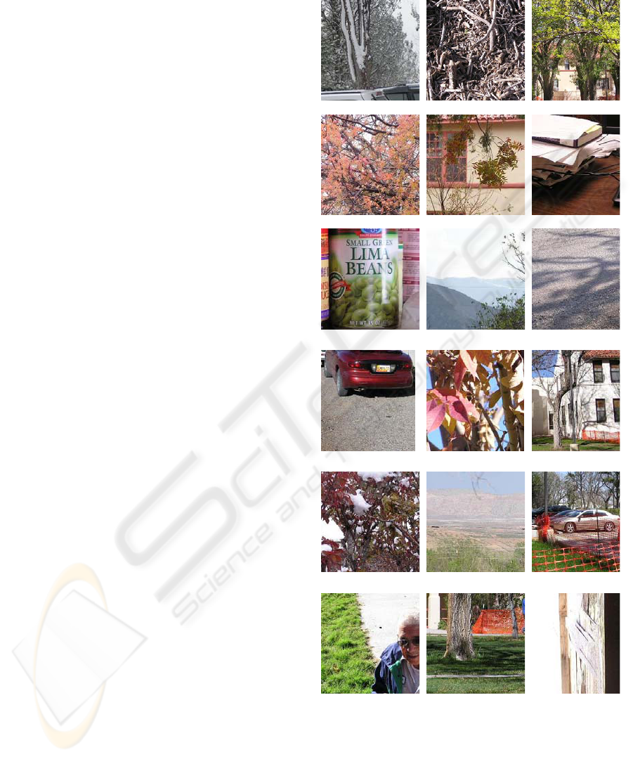
Figure 1 lists some samples of these five types of

steganograms as well as some cover samples.

5.2 Steganalysis Performance

In our experiments, besides the features set

consisting of the differences of the features from the

pre-calibrated versions and the features from the

calibrated versions, we also tested the combination

of the differences and the features from the pre-

calibrated versions. The first type of feature set is

denoted DIFF and the second type of feature set is

denoted as COMB. The original Markov approach,

denoted Markov, as well as a sub-set of Markov

features, chosen by ANOVA (the same standard to

determine the features of DIFF and COMB), are also

compared. In each experiment, 50% samples are

chosen randomly to form a training data set and the

remaining samples are tested. A Support Vector

Machine with a Radial Basis kernel Function (RBF)

(Duda et al., 2001), (Vapnik, 1998) is employed for

training and testing. In testing each type of feature

set, we do the experiment 10 times. Tables 1-1 to 1-

4 lists the average testing accuracy for each type of

feature set. Table 2 lists the testing accuracy values

of GA and WA of different feature sets.

Covers

CB stego-images

F5 stego-images

JPWIN stego-images

Steghide stego-images

MB1 stego-images

Figure 1: Some samples of the six types of JPEG images.

Generally, for an N-class classification problem,

the testing samples are m

, m

, …, m

, respectively,

corresponding to class 1, class 2, …, and class N.

The numbers of the correct testing samples are t

for

class 1, t

for class 2, …, and t

for class N. The

USING EXPANDED MARKOV PROCESS AND JOINT DISTRIBUTION FEATURES FOR JPEG STEGANALYSIS

229

general testing accuracy (GA) and weighted testing

accuracy (WA) are defined as follows:

∑

(33)

()

WA w

=×

∑

(34)

and

1/ 6, 1, 2, ..., 6

wi==

Table 1.1: The testing results of the feature set of DIFF.

Table 1.2: The testing results of the feature set of COMB.

Table 1.3: The testing results of the subset of Markov

features that is chosen by ANOVA.

Table 1.4: The testing results of the whole Markov

features.

Table 2: Average Testing accuracy (%) of GA and WA.

Feature Set GA WA

DIFF 91.3 90.6

COMB 92.1 91.4

Markov-subset 86.6 85.5

Markov 85.1 83.9

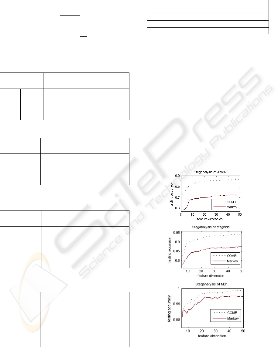
5.3 Comparison of Binary

Classification Performances

According to the results shown in table 1, the

detection performances of Markov features and the

COMB features are both close to or reach 100% in

detecting F5 and CB. We focus on the comparison

of the binary testing accuracy in detecting JPWIN,

steghide, and MB1. Since the feature selection of

support vector machine recursive feature elimination

(SVMRFE) performs well and it is applied to several

kinds of feature selection (Guyon et al., 2002), (Liu

et al. 2008a). Here we apply SVMRFE to choose

feature sets from Markov features and COMB

feature, respectively, and then apply support vector

machine to the chosen features sets. Fig. 2 compares

the detection performances.

Figure 2: Comparison of detection performances with

Markov and COMB features.

Image type JPWIN F5 CB

Steghi

MB1 Cover

Testing

accuracy

(%)

JPWIN

74.3

1.4 0.1 4.3 0.3 24.0

0.0

94.7

0.0 0.0 0.1 0.0

0.0 0.0

99.9

0.1 0.0 0.0

steghide

2.9 0.1 0.0

85.5

5.3 11.7

MB1

0.0 1.9 0.0 0.4

93.4

0.3

cover

22.9 1.9 0.0 9.8 0.9

64.0

Image type

JPWIN F5 CB

Steg

hide

MB1 Cover

Testing

accuracy

(%)

JPWIN

69.6

0.0 0.0 0.9 0.1 8.0

1.3

100

0.1 0.0 1.1 0.9

0.0 0.0

99.9

0 0.0 0.0

steghide

2.0 0.0 0.0

89.7

2.1 3.5

MB1

0 0.0 0.0 0.7

96.7

0.0

cover

27.1 0.0 0.0 8.7 0.0

87.5

Image type JPWIN F5 CB

Steg

hide

MB1 Cover

Testing

accuracy

(%)

JPWIN

69.8

0 0 0.7 0 5.6

2.1

100

0.1 0.1 1.8 1.8

0 0

99.9

0 0 0

steghide

3.2 0 0

92.3

0.7 4.0

MB1

0.1 0 0 1.2

97.5

cover

24.8 0 0 5.7 0

88.6

Image type JPWIN F5 CB

Steg

hide

MB1 Cover

Testing

accuracy

(%)

JPWIN

54.8

0.0 0.0 1.6 0.0 8.8

0.3

99.8

0.0 0.0 0.6 0.5

0.3 0.0

100

0.1 0.0 0.1

steghide

5.8 0.0 0.0

80.5

1.2 9.7

MB1

0.9 0.2 0.0 5.2

97.9

1.0

cover

38.0 0.0 0.0 12.7 0.3

79.9

ICAART 2009 - International Conference on Agents and Artificial Intelligence

230

Apparently, the detection performances on the

feature sets with COMB features are better than the

corresponding feature sets with Markov features.

6 CONCLUSIONS

In this paper, we expand the well-known Markov

features into the neighboring on the inter-blocks of

the DCT domain and the wavelet domain. We also

propose the joint distribution features of the

differential neighboring in the DCT domain and the

DWT domain, and calculate the difference of these

features from the testing image and the calibrated

version. We successfully improve the blind

steganalysis performance in multi-class JPEG

images. Since different hiding systems show

different sensitivities to the same feature set, a

method for selecting the optimal feature set is

critical to maximize detection performance, and this

topic is being addressed and it is possible to come

out in the final version of this manuscript.

ACKNOWLEDGEMENTS

The authors would like to acknowledge the support

for this research from ICASA (Institute for Complex

Additive Systems Analysis, a division of New

Mexico Tech).

REFERENCES

Duda, R., Hart, P. and Stork, D., 2001. Pattern

Classification, 2ed. New York, NY: Wiley.

Fridrich, J., 2004. Feature-Based Steganalysis for JPEG

Images and its Implications for Future Design of

Steganographic Schemes, Lecture Notes in Computer

Science, vol. 3200, Springer-Verlag, pp. 67-81.

Fridrich J., Goljan, M. and Hogeam, D., 2002.

Steganalysis of JPEG Images: Breaking the F5

Algorithm. Proc. of 5

Information Hiding Workshop,

pp. 310-323.

Guyon, I., Weston, J., Barnhill, S. and Vapnik, V., 2002.

Gene Selection for Cancer Classification using

Support Vector Machines. Machine Learning, 46(1-

3):389-422.

Harmsen, J and Pearlman, W., 2003, Steganalysis of

Additive Noise Modelable Information Hiding. Proc.

of SPIE Electronic Imaging, Security, Steganography,

and Watermarking of Multimedia Contents V. 5020,

pp.131-142.

Harmsen, J. and Pearlman, W., 2004. Kernel Fisher

Discriminant for Steganalysis of JPEG Hiding

Methods. Proc. of SPIE, Security, Steganography,

and Watermarking of Multimedia Contents VI, vol

5306, pp.13-22.

Hetzl, S. and Mutzel, P., 2005. A Graph-Theoretic

Approach to Steganography. Lecture Notes in

Computer Science, vol. 3677, pp. 119-128.

Katzenbeisser, S. and Petitcolas, F., 2000. Information

Hiding Techniques for steganography and Digital

Watermarking. Artech House Books.

Ker, A., 2005. Improved Detection of LSB Steganography

in Grayscale Images. Lecture Notes in Computer

Science, Springer-Verlag, 3200, 2005, pp.97-115.

Liu, Q. and Sung, A., 2007. Feature Mining and Nuero-

Fuzzy Inference System for Steganalysis of LSB

Matching Steganography in Grayscale Images. Proc.

of 20

International Joint Conference on Artificial

Intelligence, pp. 2808-2813.

Liu Q, Sung A, Chen, Z and Xu J, 2008a. Feature Mining

and Pattern Classification for Steganalysis of LSB

Matching Steganography in Grayscale Images. Pattern

Recognition, 41(1): 56-66.

Liu, Q., Sung, A., Xu, J. and Ribeiro, B., 2006. Image

Complexity and Feature Extraction for Steganalysis of

LSB Matching Steganography., Proc. of 18

International Conference on Pattern Recognition,

ICPR (1), pp. 1208-1211.

Liu, Q., Sung, A., Ribeiro, B., Wei, M., Chen, Z. and Xu,

J., 2008b. Image Complexity and Feature Mining for

Steganalysis of Least Significant Bit Matching

Steganography, Information Sciences, 178(1): 21-36.

Lyu, S. and Farid, H., 2005. How Realistic is

Photorealistic. IEEE Trans. on Signal Processing,

53(2): 845-850.

Marvel, L., Boncelet, C. and Retter, C., 1999. Spread

Spectrum Image Steganography. IEEE Trans. Image

Processing, 8(8): 1075-1083.

Pevny, T. and Fridrich, J., 2007. Merging Markov and

DCT Features for Multi-Class JPEG Steganalysis.

Proc. SPIE Electronic Imaging, Electronic Imaging,

Security, Steganography, and Watermarking of

Multimedia Contents IX, vol. 6505.

Sallee P, 2004. Model based steganography. Lecture Notes

in Computer Science, vol. 2939, pp. 154-167.

Sharifi K and Leon-Garcia A, 1995. Estimation of Shape

Parameter for Generalized Gaussian Distributions in

Subband Decompositions of Video. IEEE Trans.

Circuits Syst. Video Technol., 5: 52-56.

Shi, Y., Chen, C. and Chen, W., 2007. A Markov process

based approach to effective attacking JPEG

steganography. Lecture Notes in Computer Sciences,

vol.437, pp.249-264.

Vapnik, V., 1998. Statistical Learning Theory, John

Wiley.

Westfeld, A., 2001. High Capacity Despite Better

Steganalysis (F5–A Steganographic Algorithm).

Lecture Notes in Computer Science, vol. 2137, pp.289-

302.

USING EXPANDED MARKOV PROCESS AND JOINT DISTRIBUTION FEATURES FOR JPEG STEGANALYSIS

231