Geo-located Image Categorization and Location

Recognition

Marco Cristani, Alessandro Perina, Umberto Castellani and Vittorio Murino

Universit

a degli Studi di Verona, Computer Science Department

Ca’Vignal 2, 37134 Verona, Italy

Abstract. Image categorization is undoubtedly one of the most recent and chal-

lenging problems faced in Computer Vision. The scientiﬁc literature is plenty of

methods more or less efﬁcient and dedicated to a speciﬁc class of images; further,

commercial systems are also going to be advertised in the market. Nowadays, ad-

ditional data can also be attached to the images, enriching its semantic interpreta-

tion beyond the pure appearance. This is the case of geo-location data that contain

information about the geographical place where an image has been acquired. This

data allow, if not require, a different management of the images, for instance, to

the purpose of easy retrieval from a repository, or of identifying the geographical

place of an unknown picture, given a geo-referenced image repository. This pa-

per constitutes a ﬁrst step in this sense, presenting a method for geo-referenced

image categorization, and for the recognition of the geographical location of an

image without such information available. The solutions presented are based on

robust pattern recognition techniques, such as the probabilistic Latent Semantic

Analysis, the Mean Shift clustering and the Support Vector Machines. Experi-

ments have been carried out on a couple of geographical image databases: results

are actually very promising, opening new interesting challenges and applications

in this research ﬁeld.

1 INTRODUCTION

Categorizing pictures in an automatic and meaningful way is the key challenge in all

the retrieval-by-content systems [1]. Unfortunately, such problem is very hard at least

for two reasons: ﬁrst, because the meaning of a picture is an ephemeral entity, extrap-

olated subjectively by human beings; the second reason is the semantic gap, i.e., the

gap between the object in the world and the information in a (computational) descrip-

tion derived from a recording of that scene [1]. Despite this, the image categorization

research ﬁeld is one of the most fertile area in Computer Vision: an interesting, even if

dated, review can be found in [1] , where a taxonomy of the main algorithms for image

categorization and retrieval is presented. In [2], a comprehensive survey of the public

available retrieval systems is reported, and challenges and some future perspectives for

the retrieval systems are discussed in [3].

The common working hypothesis of most categorization algorithms is that images

are located in a single repository, and described with features vectors summarizing their

Cristani M., Perina A., Castellani U. and Murino V. (2008).

Geo-located Image Categorization and Location Recognition.

In Image Mining Theory and Applications, pages 93-102

DOI: 10.5220/0002340400930102

 SciTePress

visual properties. Recently, this classical framework has been improved with the use of

textual labels or tags, associated to the images. Textual labels are usually given by a

human user in order to constrain the number of ways an automatic system can categorize

an image, and suggest to the viewers the information the author of the picture wants to

communicate with it.

Very recently, this framework has been further updated with the introduction on

the market of several cheap GPS devices, mounted on the cameras. Such devices auto-

matically assign tags to the captured pictures, indicating the geographical position of

the shot. This capability charmed researchers and web designers, which understood the

potential scenario of a novel and more advanced way of sharing pictures, succeeding

and outperforming the “non-spatial” public image databases. This caused the creation

of global repositories for the geo-located images, as in Panoramio

, and the addition

of novel functionalities for the display of geo-located images in Google Earth

and

Flickr

. More speciﬁcally, the interfaces for the visualization of geo-located pictures of

Google Earth and Flickr insert over the satellite maps particular icons that indicate the

presence of a picture taken in that place, that the user can click over and enlarge. The

interface of Panoramio, exclusively suited for the maintenance of geo-located pictures,

is more structured. Pictures are visualized as thumbnails on a side frame, representing

the images geo-located on a satellite map. These interfaces allow to effectively exploit

geographical tags, permitting the users a novel way to discover places, more personal

and emotional.

As we will see in the following, this new framework discloses an innumerable set

of novel and stirring applications, that go beyond the mere visualization, which have to

be carefully explored by the researchers, and poses novel problems to be faced in the

realm of the image categorization. In this paper we analyze two of these applications.

The ﬁrst underlies and ameliorates the management and visualization of the geo-

located images. In all the interfaces, the exploration of a geo-located image database

occurs by zooming on a map in a desired location and visualizing a set of randomly

sampled images lying in the related neighborhood. This layout becomes very unattrac-

tive and uncomfortable in presence of a massive number of images, as it is currently in

all the databases considered. As a solution, an effective way to categorize geo-located

images has to be proposed, in which images have to be clustered together by taking into

account, other than the associated visual properties, also the geographical position of

acquisition.

In this way, the exploration of a geo-located database can be strongly improved.

Grouping the images for similarity and proximity permits to create geo-clusters from

which a small number of representative images can be extracted and visualized. In

this way, a better global visualization scheme can be exploited, in which each depicted

picture represents a different geographical pattern; in other words, each different zone

depicted on the map can be visualized by means of few good representatives.

Another interesting and harder issue to be dealt with is the geo-location of images,

where the goal is to infer the geographical zone in which a picture not geo-tagged

http://www.panoramio.com

http://earth.google.com/

http://www.flickr.com/

9494

has been acquired. This is useful in a entertainment context, in which one want to ﬁll

his geo-located image database with non-tagged photos. Another context could be the

forensic one, where it results essential to constrain the possible zone in which a picture

has been taken.

A similar issue was faced few years ago, under the name of location recognition

task, as an open research contest

. There, contestants were given a collection of color

images taken by a calibrated digital camera. The photographs had been taken at various

locations taken in a small city neighborhood, often sharing overlapping ﬁelds of view or

certain objects in common. The GPS locations for a subset of the images are provided.

The goal of the contest was to guess, as accurately as possible, the GPS locations of

the unlabeled images. Essentially, all the proposed resolutive approaches were based

on the reconstruction of 3D scenes owing to the registration of several images with

overlapping ﬁelds of view. Inferences on the position of non geo-located test images

was inferred by taking into account that 3D model. An example of such framework is

proposed in [4].

In our situation, the task is much harder: heterogeneous pictures taken far from each

other, at a different time of the day, have to be managed. This is a difﬁcult problem and,

to the best of our knowledge, no solutions are present nowadays. Due to the vastity

of the existent geographical varieties, it seems now reasonable to drop relying on the

geometric content encoded in the pictures, and to build a recognition technique based

on the 2D image pictorial features.

In this paper, we face the issues of the geo-clustering and geo-location recognition

of images, in the context of a large geo-located image database. We will show how us-

ing well-known techniques in the literature, such as the Probabilistic Latent Semantic

Analysis, Mean Shift Clustering and Support Vector Machine framework, strong and ef-

fective results can be achieved, proposing valuable solutions to the problems discussed

above.

The rest of the paper is organized as follows. In Sec. 2, mathematical background

notions are reported. Then, in Sec. 3, the outline of our system for geo-clustering and

geo-location recognition is detailed. Sec. 4 presents the experiments carried out on large

databases taken from Panoramio, and, ﬁnally, Sec. 5 concludes the paper, envisaging

future perspectives.

2 Mathematical Background

2.1 Probabilistic Latent Semantic Analysis

In this section, we brieﬂy review the probabilistic Latent Semantic Analysis (pLSA),

in its adaption to visual data. We describe the model using the classical terminology

of the literature on text classiﬁcation, in parallel to that regarding the image domain.

The input is a dataset of D documents (images), each containing local regions found

by interest operators, whose appearance has been quantized into W visual words [5].

Therefore, the dataset is encoded by a co-occurrence matrix of size W × D, where the

Where Am I? ICCV Computer Vision Contest, please see

http://research.microsoft.com/iccv2005/Contest/

9595

location < w, d > indicates the number of (visual) words w in the document d. The

model incorporates a single latent topic variable, z, that links the occurrence of word w

to document d. In formulae:

P (w, d) =

z=1

P (w|z)P (z|d)P (d) (1)

As a result, we have obtained a decomposition of a W × D matrix into a W × Z matrix

and a Z×D one. Each image is modeled as a probability distribution over the topics, i.e.,

P (z|d); the distribution P (w|z) encodes the topic z, as a probabilistic co-occurrence of

words. The distributions of the model, P (w|z) and P (z|d), are learnt using Expectation

Maximization (EM) [6]. The E-step computes the posterior over the topic, P (z|w, d)

and then the M-step updates the densities. This maximizes the likelihood L of the model

over the data:

L =

d=1

w=1

P (w, d)

n(w,d)

(2)

In recognition, the distribution P (w|z) is locked and EM is applied, estimating the

P (z|d) for the query images. For a deeper review of pLSA, see [7]; for an application

on scene recognition, see [8].

2.2 Mean Shift Clustering

The Mean Shift (MS) procedure is an old, recently re-discovered non-parametric den-

sity estimation technique [9, 10]; the theoretical framework of the MS arises from the

Parzen Windows technique [11], that under particular hypotheses of regularity of the

input space (independency among dimensions, see [10] for further details) estimates

the density at the d−dimensional point x as:

h,k

(x) =

k,d

i=1



x − x



(3)

where c

k,d

is a normalizing constant, n is the number of points available, and k(·)

the kernel proﬁle, that models how strongly the points are taken into account for the

estimation in dependence with their distance h (also called kernel bandwidth) to x.

Mean Shift extends this “static” expression, differentiating (3) with respect to x and

obtaining the density gradient estimator

∇

h,k

(x) =

k,d

i=1



− x







i=1





−x





i=1





−x





−x





(4)

where g(x) = k

(x). This quantity is composed by three terms: the ﬁrst is a normalizing

constant, the second one in square brackets is proportional to the normalized density

9696

gradient obtained with the kernel proﬁle k and the third one is the Mean Shift vector,

that is guaranteed to point towards the direction of maximum increase of the density.

Therefore, starting from a point x

in the feature space, and applying iteratively the MS

vector, a trajectory is produced which converges on a stationary point y

, representing

a mode of the whole feature space.

The MS procedure is widely applied to clustering issues: the ﬁrst step of the clus-

tering is made by applying the MS procedure to all the points to be analyzed {x

producing several convergency points {y

}. A consistent number of close locations of

convergence, {y

}

, indicates a mode µ

. The labeling consists in marking the corre-

sponding points {x

}

that produced the set {y

}

with the label l. This happens for all

the convergence locations l = 1, 2, . . . , L.

3 The Proposed Method

Given our set of geo-located images, the ﬁrst step toward the geo-clustering consists in

deriving a high level representation of the visual content of such images, without relying

on the geo-locations. This is achieved by the topic representation of the images given

by pLSA. Speciﬁcally, afﬁne elliptical regions are estimated for each image converted

in grey scale, constructed by elliptical shape adaptation about an interest point [12].

Each region is mapped to a circle by appropriate scaling along its principal axis and

a 128-dim SIFT descriptor is built. Then, descriptors are quantized into visual words

via K-means, and histogram word representations are built for each image. Finally, the

topic representation is obtained via EM.

Now, each image is described by a point in a Z−dimensional topic space. Adopting

an Euclidean distance and performing clustering in this space would group visually sim-

ilar images. At this point, we augment the image description by adding, for each image,

the related geo-locations. In this way, we move in an augmented space, formed by the

topic subspace and the geographical subspace, that we suppose for convenience as inde-

pendent. In other words, each image d is described with a feature vector [P (z|d), g(d)],

where g(d) ∈ R

is a couple containing its latitude and longitude values.

In order to perform clustering in the augmented domain, a multivariate kernel proﬁle is

used [10], that is:

k(x) =

u∈{z,g}



(5)

where C is a normalization constant, and h

are the kernel bandwidths for the topic

and the geographical sub-domain, respectively. This kernel is the product of two intra-

subspace kernels, and it weights in a different way each subspace, depending on the

kernel bandwidth associated.

As intra-subspace kernel k(·), we adopt the Epanechnikov kernel [10], that differ-

entiated (see Eq.4) leads to the uniform kernel g(·), i.e., a multidimensional unit sphere.

The choice of the number of topics and the values for the bandwidths is an aspect

discussed in the next section. After the clustering, we obtain a set of classes which

represent particular compact zones containing images with similar appearance.

9797

The second task, i.e. the geo-location recognition, is achieved by employing the

Support Vector Machines (SVMs) [13]. A SVM classiﬁer with Radial Basis Functions

has been trained to discriminate the clusters obtained via pLSA and MS clustering. In

the SVM training, the geographical features of the images of the different clusters are

discarded, being our task the geo-location recognition, i.e., after the training we need to

operate on features vectors in which the geographical information is not provided.

Then, for a novel image of unknown geo-location, we estimate its topic distribution

locking the P (w|z) estimated on all the data via pLSA and running the EM algorithm

(see Sec. 2.1). The obtained distribution is fed as input in the SVM classiﬁer, which has

been employed in a multi-class framework, by adopting the one-against-one policy[14].

As a result, we obtain the label of the region which the input image likely belongs to.

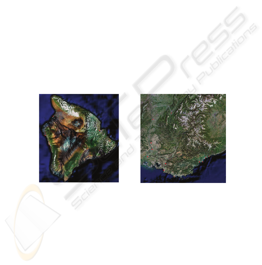
4 Experiments

To validate our framework, we built two databases considering the Hawaii Big Island

(Hawaii database), and the southern part of France (France database, see Fig.1).

Hilo

Waikoloa

Village

Kailua

Kona

Captain

Cook

Antibes

Cannes

Nice

Montecarlo

Toulon

Marseille

Aix-en-Provence

Arles

Avignon

Orange

Grenoble

Valence

4°E 5°E 6°E 7°E 8°E

46°N

47°N

48°N

49°N

20.0°N

19.5°N

19.0°N

156.0°W 155.5°W 150.0°W

Fig. 1. Geographical zones analyzed: a) Hawaii Big Island, b) Southern France.

The databases are composed by 1013 and 607 geo-located pictures, respectively, down-

loaded from Panoramio. We choose Hawaii Big Island because of its large variety of

natural scenes, ranging from mountains to sea, with volcanos, cascades and villages.

Similar considerations hold for the France database.

At ﬁrst, we perform pLSA analysis, using Z = 15 topics in both the databases.

Then, we perform Mean Shift clustering adopting a multivariate kernel (with bandwidth

9898

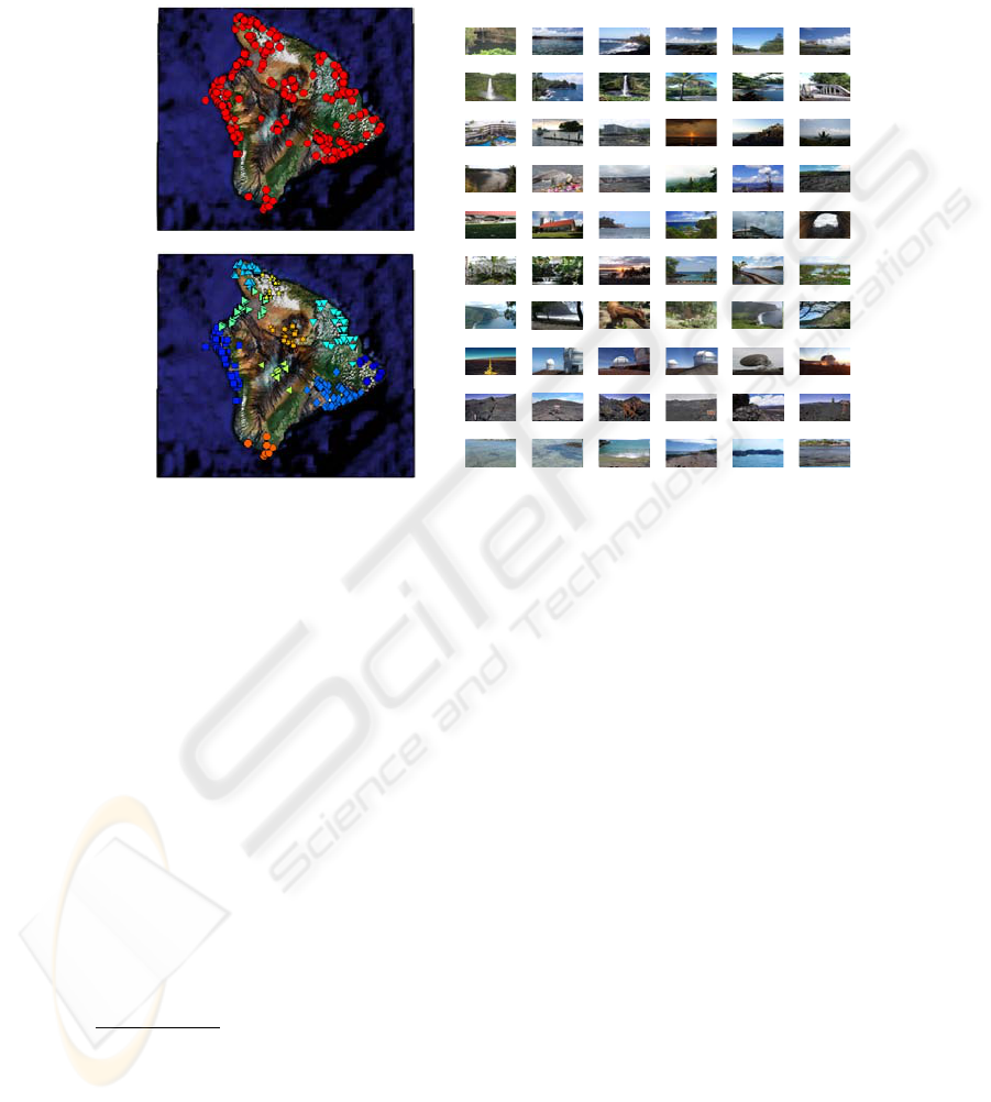
values equal to h

= 0.3 for the topic space and h

= 0.2 for the geographic space

The obtained results can be observable in Fig.2 and Fig. 3.

0.1636 |0.0192 0.2108 |0.0405 0.1885 |0.066 0.1657 |0.0877 0.2179 |0.0748 0.2176 |0.0903

0.2264 |0.00616 0.1352 |0.0211 0.1634 |0.0262 0.1968 |0.0223 0.2449 |0.021 0.1696 |0.0687

0.1432 |0.0128 0.252 |0.00956 0.2951 |0.00917 0.2944 |0.00945 0.2426 |0.0134 0.2494 |0.0143

0.229 |0.0188 0.1493 |0.0325 0.1541 |0.0358 0.1889 |0.0347 0.1614 |0.0463 0.2138 |0.0508

0.1799 |0.0127 0.2491 |0.013 0.228 |0.0424 0.2677 |0.0411 0.24 |0.0514 0.2988 |0.0416

0.2035 |0.0033 0.2946 |0.00289 0.3537 |0.0127 0.2306 |0.0331 0.1976 |0.0397

0.2301 |0.0341

0.1398 |0.894 0.1782 |0.904 0.204 |0.898 0.2042 |0.899 0.2049 |0.905

0.2039 |0.369 0.2326 |0.362 0.2339 |0.364 0.2402 |0.362 0.2922 |0.346 0.2813 |0.368

0.26 |0.393 0.2809 |0.392 0.2889 |0.391 0.3267 |0.386 0.3269 |0.389 0.4022 |0.393

0.3385 |0.825 0.3386 |0.831 0.3823 |0.882 0.5213 |0.818 0.5653 |0.848

20.0°N

19.5°N

19.0°N

20.0°N

19.5°N

19.0°N

156.0°W 155.5°W 150.0°W

0.3543 |0.840

0.1432 |0.899

Fig. 2. Hawaii database: a) location of the input photos; b) clustering results; on the right, member

images of each cluster depicted in b) are shown. On top of each image there is the Euclidean

distance between its topic distribution and the topic distribution of the cluster centroid (left); on

the top-right, the Euclidean distance between its location and the location of the centroid.

Together with the input datasets (part (a) of each ﬁgure), the clustering results (part (b)

of each ﬁgure), in the ﬁgures we show for all the clusters discovered, some member

photos depicted in ascending order w.r.t a similarity measure relative to the centroid of

the cluster. Such measure is the Euclidean distance between the topic representation of

an image and that of the centroid, multiplied by the geographical Euclidean distance.

The value of both the sub-distances are attached over the photos.

As visible in Fig.2, our clustering procedure is able to separate geographically close

zones, such as the zones 5, 6, 7, which exhibit different recurrent visual patterns (zone 5

- ﬂat coasts with buildings; zone 6 - wild beaches; zone 7 - high rocky coasts). The zone

3 is mostly formed by vegetation and cascades, zone 8 and 9 lie upon the volcanos and

zone 1, 4, and 10 represent ﬂat coasts, volcanic areas facing the sea and rocky coasts,

respectively.

Similar considerations hold for the France database. In Fig.3a the location of all the

images are shown. In Fig.3b the clustering results are shown. In the clustering, we

Regarding the parameters, changing the number of topics (we try Z = 4, . . . , 30) does not

modify drastically the quantity and the nature of the clusters obtained. The choice of the kernel

bandwidths is not critical, and easy to set.

9999

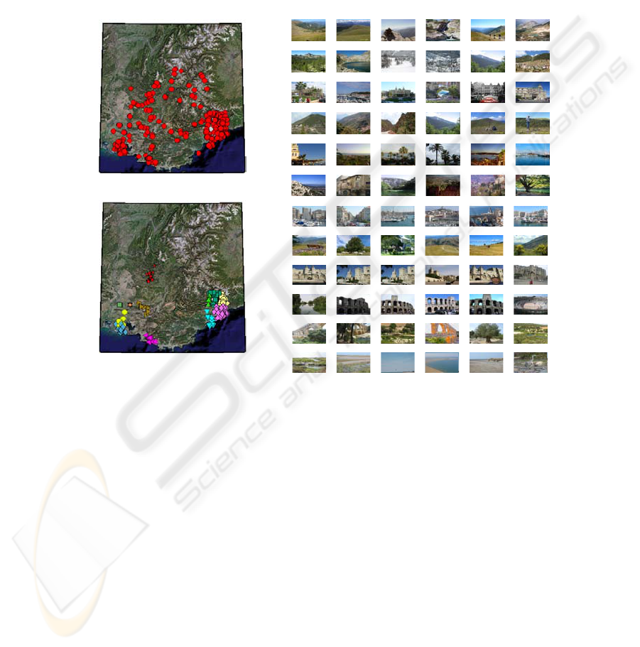
apply a size ﬁlter to discard clusters with less than 5 images. For this reason, some of

the original image locations are not shown in Fig.3 b.

In this database, the capabilities of our clustering framework are even more highlighted:

compact groups of images on the map are separated, representing highly different visual

patterns. For example, in zone 3, we can see Montecarlo; zone 5 comprehends Cannes-

Antibes. Other clusters are: zone 9 - Avignon, zone 10 - Arles, zone 11 - Pont du Gard,

zone 12 - Parc Naturel de Camargue.

0.1172 |0.01 0.1004 |0.012 0.1673 |0.00742 0.1456 |0.0103 0.1439 |0.0114 0.1354 |0.0128

0.1684 |0.0317 0.2109 |0.0317 0.1897 |0.0485 0.169 |0.0643 0.1772 |0.0648 0.1687 |0.0818

0.1458 |0.000636 0.1016 |0.000991 0.1016 |0.000991 0.1827 |0.00058 0.1587 |0.000754 0.2516 |0.000872

0.2862 |0.0131 0.1304 |0.035 0.1771 |0.0342 0.1824 |0.0346 0.181 |0.035 0.1857 |0.0357

0.1442 |0.00664 0.1836 |0.00607 0.157 |0.00734 0.2105 |0.00621 0.2053 |0.00672 0.1942 |0.00734

0.2118 |0.0134 0.3267 |0.014 0.2411 |0.0194 0.2432 |0.0191 0.2034 |0.0245 0.2742 |0.0315

0.1841 |0.0408 0.2306 |0.0405 0.1996 |0.0501 0.2184 |0.0469 0.1442 |0.0754

0.1416 |0.0418 0.131 |0.046 0.1532 |0.0605 0.1851 |0.0525 0.2341 |0.045 0.234 |0.0494

0.1161 |0.0258 0.1289 |0.0272 0.1362 |0.026 0.1642 |0.0261 0.1659 |0.0263 0.1654 |0.0269

0.1871 |0.0096 0.1645 |0.0147 0.1411 |0.0624 0.1412 |0.0624 0.2408 |0.0426 0.1612 |0.0677

0.2058 |0.0315 0.3152 |0.0207 0.3156 |0.0214 0.3162 |0.0200 0.2063 |0.0325 0.1801 |0.0405

0.1439 |0.0135 0.2568 |0.015 0.1619 |0.0723 0.1496 |0.104 0.117 |0.141 0.255 |0.0817

4°E 5°E 6°E 7°E 8°E

46°N

47°N

48°N

49°N

46°N

47°N

48°N

49°N

0.1856 |0.0406

Fig. 3. France database: a) location of the input photos; b) clustering results; on the right, member

images of each cluster depicted in b) are shown. On top of each image there is the Euclidean

distance between its topic distribution and the topic distribution of the cluster centroid (left); on

the top-right, the Euclidean distance between its location and the location of the centroid.

In order to investigate on the value added by coupling visual similarity and proximity

relation, we perform Mean Shift clustering of the images of the France dataset a) by

taking into account only the geographical position, and b) only considering the topic

distribution (Fig.4a and b, respectively), employing the same correspondent bandwidth

values adopted in the proposed method.

In the clustering performed by considering only the spatial subdomain, groups of

photos related to visually different geographical zones are fused together, as occurred

for clusters 10 and 12, and clusters 5 and 3 (see Fig. 3). In the clustering based only on

topic information, the clusters are sparse and spread out over the entire map. Here, it is

worth to note that the cluster depicted by yellow stars represent two cities, Cannes and

100100

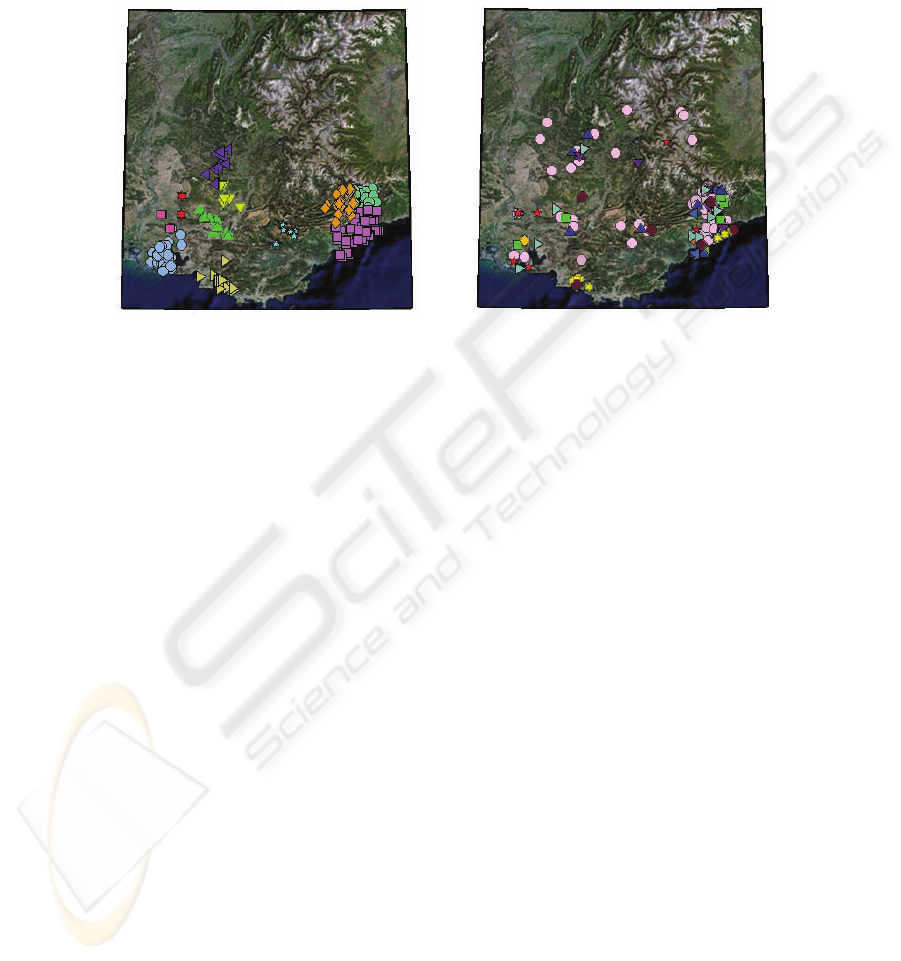
Marseille, which are geographically far but visually comparable. Similar considerations

hold also for the other clusters.

We perform the same test with the Hawaii database, obtaining similar results not shown

here due to the lack of space.

a) b)

----

Fig. 4. Clustering results by considering: a) only geographical information; b) only topic infor-

mation.

For what concerns the recognition task, we estimate the accuracy of the geo-location

recognition by performing classiﬁcation adopting the one-against-one SVMs, and cross-

validating with a Leave-One-Out policy [11], obtaining 85.24% of the accuracy on the

Hawaii database, and 75% on the France database. In this way, an unknown picture can

be located in the right geo-location, with an uncertainty given by the area of the selected

cluster: the larger the cluster, the more uncertain is the exact location where a picture

has been taken.

5 Conclusions

In this paper we propose a framework that faces successfully two novel and promising

applications in the image categorization realm, which are the geo-clustering and the

geo-location recognition. Geo-clustering consists in group together images which are

1) visually similar and 2) taken in the same geographical area. This application serves

for a more effective management and visualization of geo-located images, i.e., images

provided with geographical tags, indicating the location of the acquisition. Geo-location

recognition consists in inferring the geo-location of a picture whose provenance is un-

known, with the help of a geo-located image database. The solutions proposed with

our framework employ robust pattern recognition techniques, such as probabilistic La-

tent Semantic Analysis, Mean Shift clustering and Support Vector Machines. This work

indicates a set of future perspectives to be investigated. For example, we are currently

101101

studying a way to create of an high level description for geo-located images, such as the

one provided by the pLSA, which incorporates also the location in which the picture

has been taken. Moreover, we are studying a multi-level description, able to increase

the geographical precision with which an image can be geo-located.

References

1. Smeulders, A., Worring, M., Santini, S., Gupta, A., Jain, R.: Challenges of image and video

retrieval. IEEE Trans. Pattern Anal. Mach. Intell. 22 (2000) 1349-1380.

2. Gudivada, V.: Content-based image retrieval systems (panel). In: CSC ’95: Proceedings of

the 1995 ACM 23rd annual conference on Computer science. (1995) 274-280.

3. Lew, M., Sebe, N., Eakins, J.: Content-based image retrieval at the end of the early years. In:

CIVR 02: Proceedings of the International Conference on Image and Video Retrieval. (2002)

1-6.

4. Vision-based global localization using a visual vocabulary. In: ICRA 05: Proceedings of the

2005 IEEE International Conference on Robotics and Automation. (2005) pp. 4230-4235.

5. Junqui, W., Cipolla, R., Hongbin, Z.: Object recognition from local scale-invariant features.

Volume 2. (1999).

6. Dempster, A., Laird, N., Rubin, D.: Maximum likelihood from incomplete data via the EM

algorithm. J. Roy. Statist. Soc. B 39 (1977) 1-38.

7. Hofmann, T.: Probabilistic latent semantic indexing. In: SIGIR 99: Proceedings of the 22nd

annual international ACM SIGIR conference on Research and development in information

retrieval, New York, NY, USA, ACM Press (1999) 50-57.

8. Bosch, A., Zisserman, A., Muoz, X.: Scene classiﬁcation via plsa. In: Proceedings of Euro-

pean Conference on Computer Vision 2006. (Volume 4.) 517-530.

9. Fukunaga, K.: Statistical Pattern Recognition. second edn. Academic Press (1990).

10. Comaniciu, D., Meer, P.: Mean Shift: A Robust Approach Toward Feature Space Analysis.

IEEE Trans. Pattern Anal. Mach. Intell. 24 (2002) 603-619.

11. Duda, R., Hart, P., Stork, D.: Pattern Classiﬁcation. John Wiley and Sons (2001).

12. Mikolajczyk, K., Schmid, C.: An afﬁne invariant interest point detector. In: ECCV (1).(2002)

128-142.

13. Schlkopf, B., Smola, A.: Learning with Kernels. MIT Press (2002).

14. Hsu, C.W., Lin, C.J.: A comparison of methods for multi-class support vector machines.

IEEE Transactions on Neural Networks (2002) 415-425.

102102