RELATIVE NODES LOCALIZATION IN WIRELESS NETWORKS
USING RECEIVED STRENGTH SIGNAL VARIATIONS
Mohamed Salah Bouassida and Mohamed Shawky
Heudiasyc UMR 6599 CNRS, Universit´e de Technologie de Compi`egne
Centre de Recherche B.P. 20529, 60205 Compi`egne Cedex, France
Keywords:
Wireless Networks, Localization, Strength Signal.
Abstract:
The geographical localization of entities in a wireless network is one of the most important issues of neigh-
borhood awareness. A precise localization provides an advantage for the geographically-located services.
However, the geographical localization within a wireless network should take into account the characteris-
tics and the specificities of such environment. In this paper, we present a technique allowing a receiver to
localize a sender within its range, without additional devices, as a GPS (Global Positioning System). We use
only 3 RSSIs (Received Strength Signal Indicators) measurements, under the assumption that the sender sends
messages with the same signal strength.
1 INTRODUCTION AND
MOTIVATIONS
Wireless networks allows to connect a set of nodes in
an efficient and fast manner, using limited infrastruc-
ture support or even without any fixed infrastructure
as in ad hoc networks. The development of wireless
networks is increasing, due to the emergence of new
technologies and standards (e.g. 802.11
1
, wimax
2
)
and the exponential deployment of autonomous and
advanced equipments and devices. Furthermore, the
deployment of user-oriented services within wireless
networks brought new issues and problems. One of
the most important is the geographical localization.
Geographical localization within wireless net-
works provides important information, which can
help in several applications:
• localization of users, clients or devices
• localization for eradication of radio interferences
sources,
• localization of access points in a network,
• tracking of the motion of an entity in the network
to facilitate the local guidance based applications
...
Geographical localization techniques should take
into account the characteristics of the wireless net-
1
http://grouper.ieee.org/groups/802/11
2
http://www.wimaxxed.com
works, such as mobility and dynamicity of nodes,
low capacities in term of computation, bandwidth, en-
ergy and memory. Thus, the most suitable solution
to deal with these requirements should not use ad-
ditional devices, implying expensive overheads. In
this context, we propose in this paper a relative lo-
calization technique within wireless networks, based
on the received strength signal variations, without any
knowledge about the environment (pre-established ra-
dio map). Our localization technique is dedicated to
operate within wireless networks, composed of small
number of nodes, even 2 nodes only, for low-speed
oriented applications (eg. walking-speed oriented ap-
plications).
To present our contributions, this paper is struc-
tured as follows. Section 2 presents related works
concerning geographical localization in wireless net-
works. In section 3, we describe our technique to
locate a non mobile transmitter within LoS environ-
ment. In Section 4, we show how to calibrate the
signal attenuation model within LoS environment, to
produce the most exact RSSI measurements Section
5 presents the typical applications integrating our lo-
calization technique: a tracking mechanism of nodes
within wireless network and a combined positioning
technique using identified beacon nodes. Section 6
presents analysis and results, and finally section 7
concludes this paper and presents our future work.
195
Salah Bouassida M. and Shawky M. (2008).
RELATIVE NODES LOCALIZATION IN WIRELESS NETWORKS USING RECEIVED STRENGTH SIGNAL VARIATIONS.
In Proceedings of the International Conference on Wireless Information Networks and Systems, pages 195-202
DOI: 10.5220/0002020601950202
Copyright
c
 SciTePress

2 RELATED WORK
The GPS (Global Positioning System) (Hofmann-
Wellenhof et al., 1997; Stoleru et al., 2004) is the
most known localization technique. Each entity holds
a sensor which receives and process signals from a
satellite constellation, to define a 3-dimensional lo-
calization having an error margin evaluated to 10m
to 20m. This localization method is widely used by
mobile devices. However, it still expensive to deploy
within wireless networks, in addition to the low relia-
bility of the satellite signal reception indoors.
During the last years, were developed several
localization techniques in wireless networks. We
present in this section some of them, divided into two
approaches: range free and range based techniques
(He et al., 2003).
2.1 Range Free Localization Techniques
In these techniques also called topologicaltechniques,
no physical measurements are used. The localization
is only based on the data links established by the node
to situate, with its neighbors. Within these techniques,
reference nodes called beacons are chosen, having
self localization capabilities such as GPS. The mech-
anisms belonging to this approach are as follows:
• Centroid algorithm (Bulusu et al., 2000): a node
that needs to localize itself, computes an average
of the coordinates of the reference nodes that it
receives. The obtained localization may have a
large error margin.
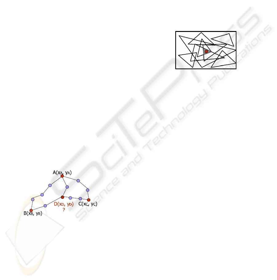
Figure 1: DV-HOP localization technique.
• DV-HOP (Niculescu and Nath, 2001b) each node
estimates its position via the diffused coordinates
of the beacons nodes, the number of hops to reach
these nodes and the average size of one hop within
the network. This average size is estimated by
the beacon nodes and diffused within the net-
work. Figure 1 illustrates this localization tech-
nique. The node D to situate, is at 2 hops from
the beacon A (of size average
A
), 2 hops from the
beacon B (of size average
B
) and 3 hops from the
beacon C (of size average
C
).
The main disadvantageof this technique is that the
average size of one hop in the network could not
be determined precisely. To solve this problem,
another technique called Amorphus Positioning
(Nagpal et al., 2003) is deduced from DV-HOP,
while taking into account the density of nodes in
the network.
• PIT (He et al., 2003): each node within the
network evaluates its position according to the
formed triangles between the beacon nodes. Each
result allows to refine the computed localization.
This technique can produce only estimations of
the node localization (cf. Figure 2).
Figure 2: PIT localization technique.
2.2 Range based Localization
Techniques
These techniques also called topographic techniques
are based on physical measurements data, carried out
for each wireless link established between the node
to localize and its environment. The mechanisms be-
longing to this approach are presented in the follow-
ing:
• Angle of Arrival (AOA): the localization of a node
is computed by a triangulation using the angles
of reception according to three beacon nodes (cf.
Figure 3). The APS (Ad-hoc positioning system)
(Niculescu and Nath, 2001a) technique uses the
AOA localization within wireless networks. APS
proposes a method for all nodes to determine their
orientation and position in an ad hoc network,
where a fraction of nodes have positioning capa-
bilities (GPS) and under the assumption that each
node has the AOA capability. These requirements
make APS restricted to a specific context of wire-
less ad hoc networks.
• Time of Arrival (TOA): the localization of nodes
is computed via the propagation times between
the concerned entity and the beacon nodes. Both
one-way propagation time and round trip time are
used. The Cricket (Priyantha et al., 2000) tech-
nique uses the TOA localization mechanism, in
addition to the combination of the RF and ul-
trasound hardware to enable a sensor, attached
to each node, to compute the distance to beacon
WINSYS 2008 - International Conference on Wireless Information Networks and Systems
196

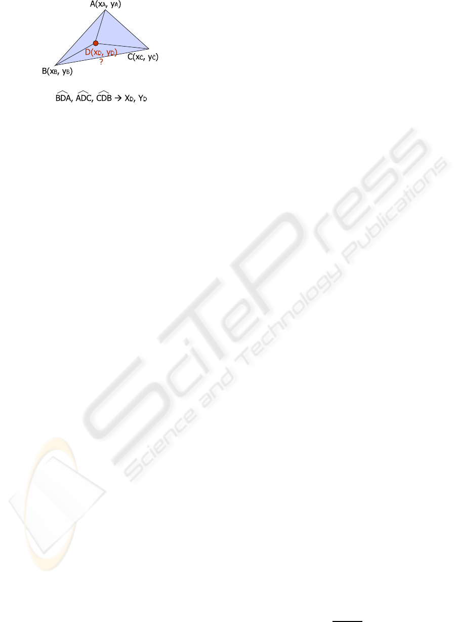
Figure 3: AOA localization technique.
nodes as follows: a beacon node sends informa-
tion about the space over RF, together with an ul-
trasound pulse. A listener receives the RF mes-
sage and then the ultrasound pulse, which arrives
later due to the speed difference between RF and
ultrasound waves. The time difference between
the reception of the RF message and the ultra-
sound signal determines the distance to the bea-
con node.
• Time Difference of Arrival (TDOA): the local-
ization of nodes within the network is carried
out according to the relative moments of detec-
tion of a common event (such as ultra-sound mes-
sage reception). This technique supposes a syn-
chronization between the nodes, hardly applicable
within wireless networks, due to their lack of fixed
infrastructure. The Pushpin technique (Broxton
et al., 2005) is a typical example of TDOA tech-
nique.
• Received Signal Strength Indicator (RSSI): dis-
tance between nodes is estimated according to an
attenuation model of the received signal strength
with distance. Path loss models represent the dif-
ference in dB in signal strength between trans-
mitter and receiver via RSSI measurements. The
most known model to evaluate the path loss is the
Friis Free Space Path Loss Model (described in
section 3).
The localizations techniques presented above al-
low a node within a wireless network to situate itself,
according to reference nodes in the network (range
free techniques), or to physical measurements car-
ried out between the node and its environment (range
based techniques). The majority of these approaches
needs additional configurations or equipments which
make them restricted to a specific wireless network
context.
To deal with this inconvenient, we elaborate a fast
and reliable localization technique based on the RSSI
measurements, to operate within small wireless net-
works, without the need of any additional device or
configuration (cf. section 3).
3 RELATIVE LOCALIZATION OF
A NON MOBILE
TRANSMITTER WITH LOS
ENVIRONMENT
We propose in this section a technique allowing a
mobile receiver to localize a fixed sender within its
range, with only 3 RSSI measurements, in LoS (Line
of Sight) environment and assuming that sent mes-
sages are with the same signal strength.
The path loss model we use to evaluate the dis-
tance between a sender and a receiver is the Friis Free
Space Path Loss Model, which represents the signal
attenuation when there is a clear line of sight between
the transmitter and the receiver. This model stipulates
that:
PLfs(d)[dB] = 20.log
10
(4πd/λ)
Where:
• λ is the wavelength of the propagation wave. λ
is evaluated as λ = c/ f, c is the light speed
(3.10
8
m/sec) and f is the frequency of the sig-
nal. For 802.11g (the dominating frequency is
f = 2.4Ghz), λ = 0.125m,
• d is the distance between the transmitter and the
receiver.
To generalize the previous equation with any dis-
tance d, we use the following path loss expression,
which integrates a received power reference point
(d0). We can choose d0 = 1m without loss of gen-
eralization:
PL(d)[dB] = 2.PLfs(d0)[dB] + 10.n.log
10
(d/d0)
Where n is the path loss exponent which repre-
sents the increase of path loss with increase in the
distance between the transmitter and the receiver. For
free space, n is equal to 2, but it would be better to
calibrate this parameter, depending on each network
characteristics.
Figure 4 illustrates a typical example where the
receiver needs to localize the sender by determining
the angle β between them. For that, the receiver starts
by evaluating the received strength from the sender,
at positions P
1
and P
2
. The distance between these
positions is L. Then, using the Friis path loss model,
the receiver can evaluate the distances d
1
and d
2
at
positions P
1
and P
2
.
We suppose that the distance x between the re-
ceiver and the sender is equal to the average between
the distances d
1
and d
2
, where d
1
,d
2
>> L.
x =
d
1
+ d
2
2
RELATIVE NODES LOCALIZATION IN WIRELESS NETWORKS USING RECEIVED STRENGTH SIGNAL
VARIATIONS
197

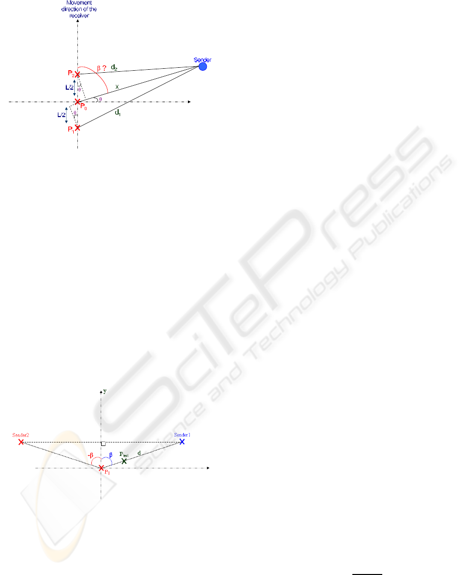
Figure 4: Evaluation of the angle between the sender and
the receiver.
The followingrelations allow computingthe angle
β:
d
2
1
= (x+ L/2.sinΘ)
2
+ (L/2.cosΘ)
2
d
2
2
= (x− L/2.sinΘ)
2
+ (L/2.cosΘ)
2
⇒ d
2
1
− d
2
2
= 2.L.x.sinΘ
⇒ sinΘ = (d
2
1
− d
2
2
)/2Lx
⇒ β = arccos((d
2
− d
1
)/L)
Let the coordinates of the receiver at the posi-
tion P
0
be (x
0
,y
0
), and the coordinates of the sender
(x
s
,y
s
). Because of cos(x) = cos(−x), two localiza-
tions of the sender are possible, verifying the equation
β = arccos((d2 − d1)/L). From Figure 5, we show
that:
x
s
= x
0
+ d.sinβ or x
s
= x
0
− d.sinβ
y
s
= y
0
+ d.cosβ or y
s
= y
0
+ d.cosβ
Figure 5: Localization of the sender using the angle β.
To be able to decide which position to choose for
the sender, the receiver can measure the received sig-
nal strength from the sender, in the direction of one
of the two localizations. Depending on the increase
or the decrease of the received signal strength, the
receiver decides which localization to choose for the
sender. In figure 5, if the received signal strength in-
creases at position P
test
, the sender is at the localiza-
tion 1; otherwise, it is at the position 2.
3.1 Advantages of Our Localization
Technique
The main advantages of our localization technique are
the following:
• No additional equipment has to be added to the
wireless nodes to situate. Our localization tech-
nique uses only the history of received signal
strength, to deliver a reliable and fast localization
estimation.
• The node which wants to localize itself can move
within the network and does not need to be fixed,
as others localization techniques based for exam-
ple on triangulation mechanisms.
• The higher is the number of measurements of the
received signals strength, the more is the localiza-
tion precision. Indeed, the measurements of RSSI
can calibrate the path loss attenuation model used
to compute the distance between the sender and
the receiver (cf. section 4).
• Our localization technique can be integrated to
other advanced mechanisms. We present in Sec-
tion 5 a tracking technique of a node within wire-
less networks and a combined positioning tech-
nique using identified beacon nodes.
4 CALIBRATION OF THE
EXPONENT LOSS FACTOR
WITHIN LoS ENVIRONMENT
To avoid errors on the RSSI measurements, we should
calibrate the exponent loss factor n used in the Friis
Loss equation presented in section 3. With d0 = 1,
we have PL(d)[dB] = 80 + 10n.log
10
(d). Thus, the
distance d and the loss factor n are computed as fol-
lows:
d = 10
(PL(d)[dB]−80)/10n
n = (PL(d)[dB] − 80)/10.log
10
(d)
To calibrate n, we use a second formulation of the
Friis Model, which stipulates that: P
r
/P
t
= (λ/4πd)
2
;
where P
r
is the received signal strength and P
t
is
the transmitted signal strength. For two successive
received signals from a transmitter, we show that
P
r1
/P
r2
= (d
2
/d
1
)
2
. We thus have:
d
2
= d
1
.
p
P
r1
/P
r2
Our calibration algorithm, illustrated in Figure 6,
consists of computing the distance between a trans-
mitter and a receiver as the average between the two
WINSYS 2008 - International Conference on Wireless Information Networks and Systems
198

Figure 6: Calibration of the path loss factor.
values produced by using the two formulation of the
Friis Loss equation. The exponent loss factor n is
then computed as a function of the computed aver-
age distance. We add to our calibration algorithm a
trust level, which represents the number of calibra-
tions carried out by a node in the network.
5 TYPICAL APPLICATIONS OF
OUR POSITIONING
TECHNIQUE
5.1 Tracking of a Mobile Node Within
Wireless Networks
Our objective is to allow a mobile node A to track
another mobile node B within the network, by only
using RSSI measurements (cf. Figure 7).
Figure 7: Tracking of a node in the network.
To compute the angle between two mobile nodes,
we suppose that the flow of data sent by a node to an
other is sufficiently high to consider that the motion
of the two nodes can be divided into small sequential
segments (each of the two nodes moves in its turn).
We can thus use the localization technique described
in section 3 to compute the angles α and β between
the two nodes A and B.
Nodes A and B send periodically and mutually the
angles α and β between them, as is illustrated in Fig-
ure 7, computed via our localization technique pre-
sented above. To track node B, the node A should
deviate its direction by π− α− β.
We are currently working on a two-nodes encoun-
tering application within a wireless network. This
application consists of bringing together two mobile
nodes, which periodically send to each other their lo-
calization information. Each node compute the angle
between its direction and the direction of the other
node and deviates its direction in order to encounter
the other node, while decreasing the distance between
them.
5.2 Combined Localization using
Identified Beacon Nodes
We present in this section a technique allowing a
node to identify its trajectory within a wireless net-
work, where beacon nodes are chosen having local-
ization capability by GPS (cf. Figure 8). The bea-
con nodes sends periodically localization messages to
their neighbors in one hop (TTL=1). Each localiza-
tion message contains the coordinates of the beacon
node and the time of transmission.
Figure 8: Identification of the trajectory of a node in the
network.
The mobile node, moving within the wireless net-
work, receives the localization messages sent by the
beacon nodes allowing it to identify its trajectory ac-
cording to the following algorithm:
while ()
Receive Localization-Message from beacon node i
if Receive 3 Localization-Messages from the
same node i
Compute the localization according to the beacon
node i
Store the localization within a positions history
RELATIVE NODES LOCALIZATION IN WIRELESS NETWORKS USING RECEIVED STRENGTH SIGNAL
VARIATIONS
199

end if
if Trajectory Identification
Linearization of the node trajectory using
the positions history
end if
end while
To validate the applicability of our main contribu-
tions presented above, we present in the next section
analysis and simulations we have done to calibrate
the parameter L of our localization technique, simu-
late our calibration algorithm and finally evaluate the
localization error margin depending on the different
parameters of our approach.
6 ANALYSIS AND SIMULATIONS
6.1 Analytical Results
In the new localization technique presented in section
3, the parameter L should be well chosen to improve
the reliability and the exactness of the results. Figure
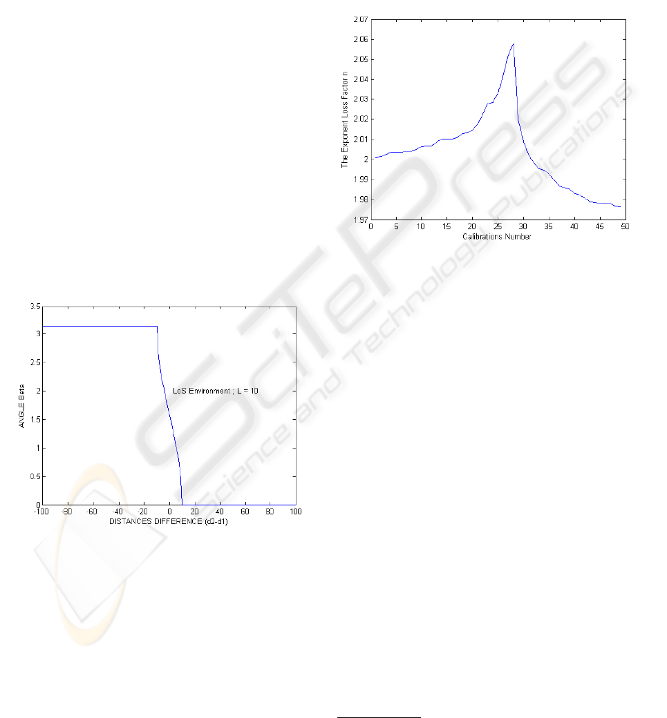
9 (L = 10) shows the angle β, computed as a function
of the difference between the two distances d
1
and d
2
.
We show for example that when d
1
= d
2
, the sender
is at 90
o
from the receiver.
Figure 9: Angle β by (d2-d1) with LoS environment and
L=10.
The choice of L is important to have a fast and
reliable measurement of the angle β. Indeed, a large
L compared to d
1
and d
2
, allows more opportunities
to measure exactly the angle β (the interval [−L,L]
is large). On the other hand, measuring the received
signal with a small L is faster and easier.
From Figure 9, we show that to enhance the ex-
actness of our localization technique, we have to en-
sure the following inequality: |d2 − d1| < L. Let’s
T
measure
define the time measurement period (the time
between two RSSI measurements) ; and V is the max-
imum speed of the receiver. The distances differ-
ence (|d2 − d1|) should thus be limited to V.T
measure
.
Hence, the parameter L should be chosen as follows:
L > V.T
measure
For example, for T
measure
= 1sec and for V = 10km/h
(average walking speed), L should be equal to 3m.
Figure 10: Calibration of the n loss factor.
In a second step of our analysis, our objective is
to verify our calibration mechanism of the n loss fac-
tor n, presented in section 4. We choose a simulation
example, in which we start initially by n = 2, the re-
ceived signal strength Pr = 150w and the signal loss
PL = 70w. We calibrate the n loss factor 50 times
according to the algorithm presented in Figure 6. At
each calibration, we add a random value (between 0
and 1) to the value of PL. The result of our verifica-
tion example is presented in Figure 10. We show in
this Figure how the exponent loss factor can be ad-
justed depending on the RSSI measurements.
6.2 Simulation Results
In this section, we use the network simulator NS2
3
to simulate our localization mechanism, described in
section 3.
Our simulation parameters under NS2 are as fol-
low:
• channel type: wireless,
• propagation model: Free Space,
• MAC protocol: 802.11,
• antenna model: omni-directional,
• number of nodes: 2,
3
http://www.isi.edu/nsnam/ns/
WINSYS 2008 - International Conference on Wireless Information Networks and Systems
200

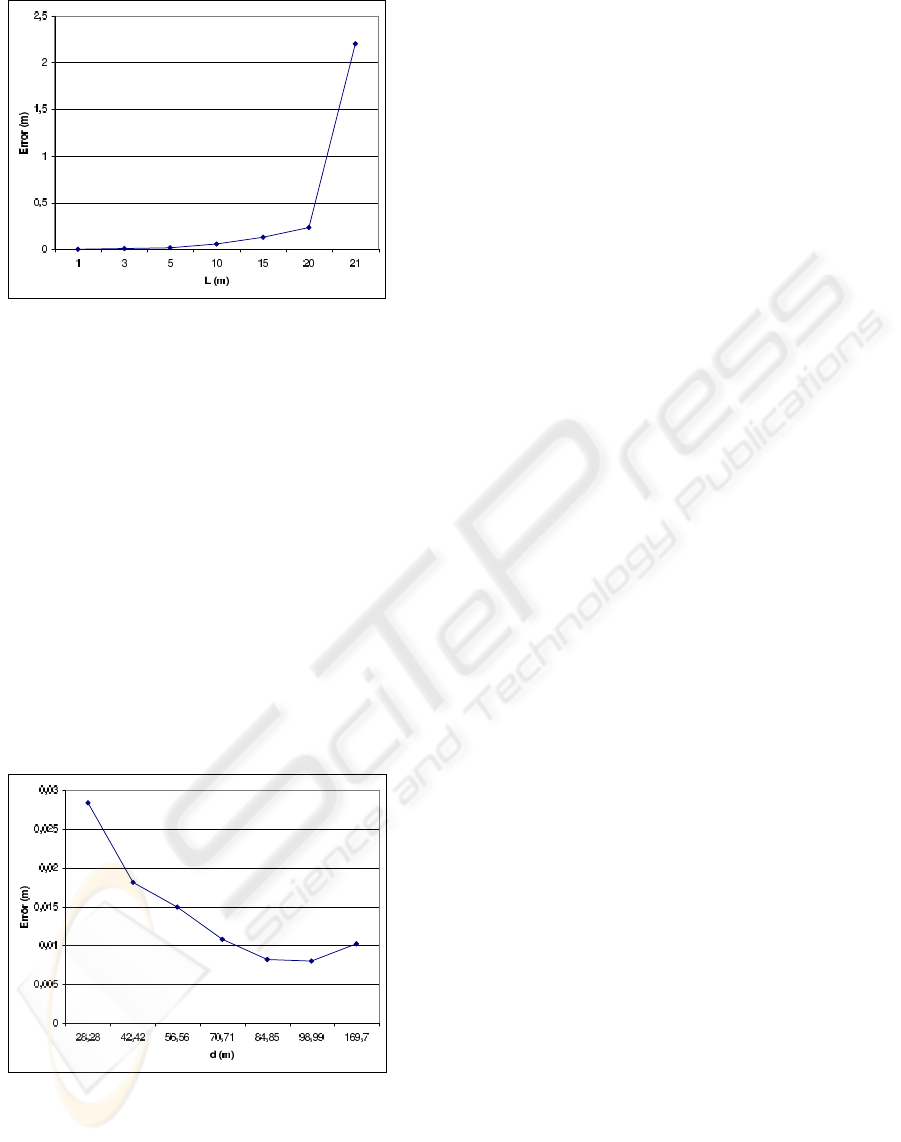
Figure 11: Localization Error by L (d = 180.27m).
• traffic: node 1 sends a CBR traffic to node 0,
which receives these packets, evaluate their RSSIs
and compute the distance to reach node 1.
We carried out simulations to evaluate the local-
ization error of our approach. In a first step, we eval-
uate the localization error according to the distance L
between the two positions P
1
and P
2
, the distance d is
fixed to 180.27 (cf. Figure 11). Then, we evaluate the
localization error according to the distance d, while
fixing the L parameter (L = 3m) (cf. Figure 12).
We show in Figure 11 that the localization error
is strongly dependant on the parameter L. The small-
est the parameter L is, the smallest is the localization
error. For L = 3m, the localization error is equal to
0.0043m. However, we cannot decrease indefinitely
the parameter L in order not to distort the RSSI mea-
surements.
Figure 12: Localization error by the distance d (L = 3m).
Figure 12 shows that the localization error is de-
pendant on the distance between the sender and the
receiver, with a fixed L. We conclude that to have
a small localization error, the parameter L should be
much smaller then the distance d. In addition, we
have used this hypothesis to compute the angle β be-
tween the sender and the receiver (cf. Section 3).
7 CONCLUSIONS AND FUTURE
WORK
We presented in this paper a new localization tech-
nique, based only on the RSSI measurements. This
technique allows a mobile node to compute the po-
sition of a fixed node in the network, by evaluating
the variation of the received signal strength of three
messages sent by this node. In a second step, we pre-
sented a calibration mechanism of the Friis attenua-
tion model within LoS environment. This mechanism
consists of calibrating the exponent loss factor n at
each achieved RSSI measurement. We deduced from
our positioning technique a tracking mechanism and a
combined localization technique using identified bea-
con nodes.
To validate our contributions, we carried out anal-
ysis and simulations to calibrate the different parame-
ters of our localization technique. We showed that the
choice of the parameter L is very important to mini-
mize the computed localization error.
The establishment of secure communications
within wireless networks remain a key issue be-
cause of the characteristics and the vulnerabilities of
such environment (Bouassida, 2006; Bouassida et al.,
2006). In this context, other research works in our
team are dealing with the assessment of security of
messages using signal characteristics. We envisage
to adapt our technique in order to obtain a ”distin-
guishability” degree between two nodes by analyzing
strength variations. This will contributeto detect sybil
nodes created by a malicious one.
REFERENCES
Bouassida, M. S. (2006). S´ecurit´e des communications de
groupe dans les r´eseaux ad hoc. PhD thesis, Univer-
sit´e Henry Poincar´e, Nancy France.
Bouassida, M. S., Chrisment, I., and Festor, O. (2006).
Group Key Management within Ad Hoc Networks. In-
ternational Journal of Network Security. Accepted for
Publication.
Broxton, M., Lifton, J., and Paradiso, J. (2005). Localiz-
ing a sensor network via collaborative processing of
global stimuli. In Proceedings of the Second Euro-
pean Workshop on Wireless Sensor Networks, pages
321–332, Istanbul, Turkey.
Bulusu, N., Heidemann, J., and Estrin, D. (2000). Gps-less
low cost outdoor localization for very small devices.
IEEE Personal communication Magazine, 7(5):28–
34.
RELATIVE NODES LOCALIZATION IN WIRELESS NETWORKS USING RECEIVED STRENGTH SIGNAL
VARIATIONS
201

He, T., Huang, C., Blum, B., Stankovic, J., and Abdelzaher,
T. (2003). Range-free localization scheme for large
scale sensor networks. In MobiCom, pages 81–95.
Hofmann-Wellenhof, B., Lichtenegger, H., and Collins, J.
(1997). Global Positioning System: Theory and Prac-
tice. Springer-Verlag, 4th edition.
Nagpal, R., Shrobe, H., and Bachrach, J. (2003). Orga-
nizing a global coordinate system from local informa-
tion on an adhoc sensor network. In 2nd International
Workshop on Information Processing in sensor net-
works (IPSN’03), Palo Alto.
Niculescu, D. and Nath, B. (2001a). Ad-hoc positioning
system (aps) using aoa. In Proceedings of IEEE IN-
FOCOM, pages 1734–1743.
Niculescu, D. and Nath, B. (2001b). Ad-hoc positioning
systems (aps). In Proceeding of IEEE Globecom,
pages 2926–2931.
Priyantha, N., Chakraborty, A., and Balakrishnan, H.
(2000). The cricket location-support system. In 6th
ACM MOBICOM, Boston, MA.
Stoleru, R., He, T., and Stankovic, J. A. (2004). Walking
gps: A practical solution for localization in manu-
ally deployed wireless sensor networks. In LCN ’04:
Proceedings of the 29th Annual IEEE International
Conference on Local Computer Networks (LCN’04),
pages 480–489, Washington, DC, USA. IEEE Com-
puter Society.
WINSYS 2008 - International Conference on Wireless Information Networks and Systems
202