SIGNAL-DEPENDENT ANALYSIS OF SIGNALS SAMPLED BY
SEND ON DELTA SAMPLING SCHEME
M. Greitans and R. Shavelis
Institute of Electronics and Computer Science, 14 Dzerbenes str., Riga, Latvia
Keywords:
Signal driven A/D conversion, send on delta sampling scheme, spectral analysis, signal dependent transforma-
tion.
Abstract:
Interest in the application of signal driven sampling schemes is increasing as they offer various advantages
over traditional sampling. The paper describes the principles and discusses the properties of sampling, which
is based on the send-on-delta concept. In such a way, it is possible to decrease the sampling density, and since
the samples are placed non-equidistantly it is possible to suppress the distortion due to frequency aliasing. The
non-uniform location of samples requires an advanced processing method. The paper discusses the spectral
estimation, which is based on the use of a bank of minimum variance filters. To improve the resolution
and accuracy, iterative updating of autocorrelation matrix is used. The results of simulations are presented.
The use of an iterative algorithm allows correcting spectral estimation even if the mean sampling density is
several times less than the Nyquist criterion. The proposed approach can be of interest for distributed wireless
data acquisition in remote sensing systems, because it allows the amount of transmitted data to be decreased
considerably.
1 INTRODUCTION
Regarding signal sampling procedures, generally, the
signal can be approximated with fewer samples per
interval using appropriate non-equidistantly spaced
samples than using a uniform sampling procedure,
where the sampling frequency is defined taking into
account only the highest signal component. The prob-
lem of processing non-uniformly sampled signals has
quite a long history. However it typically deals with
cases, where non-uniformity is introduced in a delib-
erate or deterministic way. Intuitively speaking, the
sampling flow has to reflect the local properties of
the signal. For example, it is more efficient to sam-
ple the low frequency regions at a lower rate than
the high frequency regions. A special class of non-
uniform sampling is derived if the sampling process
is driven by the signal itself this is so called signal
dependent sampling. The popular types of signal-
dependent sampling are zero crossing, reference sig-
nal crossing, level crossing or send-on-delta concepts.
In the paper, sampling based on the send-on-delta
(SoD) concept is employed. The motivation of such
a choice is based on three key aspects. Firstly, it is
signal dependent sampling, which offers various ad-
vantages over traditional uniform sampling (Hauck,
1995). Secondly, this sampling scheme can be sim-
ply implemented in hardware, because it guarantees
a certain minimal interval between samples. Thirdly,
the non-uniformity in sampling provides the possibil-
ity of suppressing frequency aliasing (Masry, 1978),
and therefore the SoD scheme can be used to reduce
the sampling density in comparison with the Nyquist
rate. The properties of send-on-delta sampling will be
discussed in Section 2.
The reason, why the SoD sampling is not
widespread in practice, lies in the fact that such digi-
tized signals can not always be successfully processed
using standard algorithms. One of the main process-
ing tasks is the estimation of the signal spectrum.
In the case of uniform sampling, the Nyquist crite-
rion determines the minimum sampling rate, which
must be fulfilled in order to avoid frequency aliasing.
To estimate the spectrum of a non-uniformly sam-
pled signal, an advanced signal processing method
is required, especially in the cases where the sam-
pling density can be below the Nyquist criterion.
The paper discusses the spectrum estimation method
that is based on signal-dependent transform (Greitans,
2005), which uses the minimum variance filter prin-
ciple and provides spectral estimation with high reso-
lution and accuracy. The algorithm will be described
in Section 3, and simulation results will be shown in
Section 4.
125
Greitans M. and Shavelis R. (2008).
SIGNAL-DEPENDENT ANALYSIS OF SIGNALS SAMPLED BY SEND ON DELTA SAMPLING SCHEME.
In Proceedings of the International Conference on Signal Processing and Multimedia Applications, pages 125-130
DOI: 10.5220/0001937201250130
Copyright
c
 SciTePress

2 SEND-ON-DELTA SAMPLING
According to the level-crossing (LC) concept the sam-
pling is triggered if the input signal crosses any of the
fixed quantization levels (Allier and Sicard, 2003).
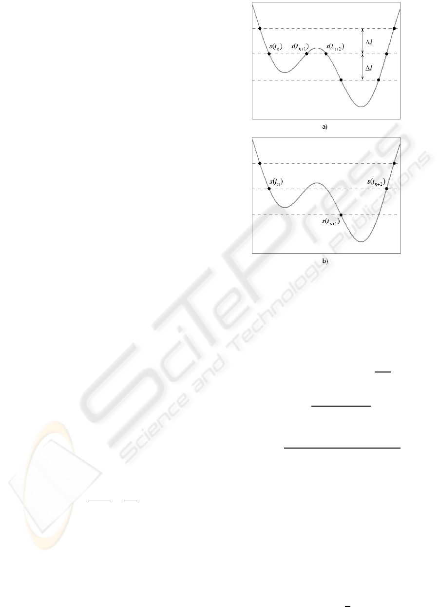
The principle of LC sampling is illustrated in Fig-
ure 1a. The number of samples captured depends
on signal itself (Mark and Todd, 1981), (Greitans,
2006). The minimum distance ∆t
min
= min(∆t
n
),
where ∆t
n
= t
n+1
−t
n
, between the sampling points t
n
can be very small and thus the analog-to-digital (A/D)
converter can not ensure all the samples are captured
due to the limited performance of electronic compo-
nents.
2.1 Sampling Scheme
The situation changes in case of send-on-delta sam-
pling scheme, according to which the sampling is trig-
gered if the signal deviates by defined value ∆l > 0,
called the threshold, or delta (Miskowicz, 2006). The
principle of SoD sampling is shown in Figure 1b.
There is a constant difference equal to ∆l between
consecutive signal values
|s(t
n+1
) −s(t
n
)| = ∆l, (1)
where s(t
n
) is a signal sample at the time instant t
n
.
The threshold ∆l determines the resolution of signal
observations. The smaller ∆l, the higher resolution of
input signal tracking.
2.2 Minimum Sampling Interval
Obviously, N
LC
≥ N
SoD
, where N
LC
and N
SoD
are the
numbers of samples captured by using respectively
LC and SoD sampling schemes. The minimum dis-
tance ∆t
min
in case of SoD depends on ∆l and on the
spectral properties of the signal. For example, if a
single sinusoid
s(t) = Asin(2πft + ϕ) (2)
is sampled, then the minimum distance, if ω = 2πf,
is
∆t
min
≥
∆l
2Aπ f
=
∆l
Aω
(3)
as the maximum value of derivative is Aω.
Another example is the signal with constant power
spectral density
P( f) =
(
A
2
for |f| ≤ f
max
0 elsewhere
. (4)
To achieve the maximum slope of such a signal the
phase has to be the same at all frequencies. In this
Figure 1: Signal dependent sampling based on a) level-
crossing and b) send-on-delta concepts.
case the iverse Fourier transform is described by sinc
function:
s(t) = 4Aπf
max
sinc(2π f
max
t) (5)
To estimate the maximum value of derivative of s(t),
lets first look at signal u(t) = sinc(t) =
sin(t)
t
. The first
and second order derivatives of u(t) are:
u
′
(t) =
tcos(t) −sin(t)
t
2
(6)
and
u
′′
(t) =
−t
2
sin(t)−2tcos(t) + 2sin(t)
t
3
(7)
To estimate the maximum value of (6), we solve the
equation
u
′′
(t) = 0 (8)
From (8) it follows, that t 6= 0 and
tcos(t) = sin(t) −0.5t
2
sin(t) (9)
Lets say we have the solution of (9) if t = t
0
, then
inserting (9) into (6) gives:
u
′
(t
0
) = −0.5sint
0
(10)
It means, that the maximum value of u
′
(t)
u
′
(t)
max
≤
1
2
(11)
SIGMAP 2008 - International Conference on Signal Processing and Multimedia Applications
126

In turn, the derivative of s(t) can be expressed as
s
′
(t) = 8Aπ
2
f
2
max
(sinc(t))
′
= 8Aπ
2
f
2
max
u
′
(t). (12)
From (12) and (11) follows, that the maximum value
of s
′
(t)
s
′
(t)
max
≤ 4Aπ
2
f
2
max
= Aω
2
max
(13)
and the minimum distance
∆t
min
≥
∆l
Aω
2
max
. (14)
2.3 Sampling Density
Due to the signal-dependent nature of SoD, the sam-
pling density depends on the statistical characteristics
of the signal. If l
k
are the values of quantization lev-
els crossed by the signal, then in case of only one
quantization level l
1
the number of SoD samples cap-
tured will be N
l
1
= 1. In case of two levels l
1
and l
2
the numbers of samples N
l
1
= N
l
2
as every next sam-
pling is triggered by crossing the quantization level,
which differs from the previous one. If we start the
numbering of levels from the lower one, then in case
of three levels l
1
, l
2
and l
3
the numbers of samples
N
l
1
= N
l
2
−N
l
3
since SoD captures at the second level
is also caused by the third level. In general, if there
are K quantization levels, then
N
l
1
=
K
∑
k=2
(−1)
k
·N
l
k
(15)
Now let us first discuss the case, when the sig-
nal is sampled by level crossing. For a single sinusoid
Asin(2π ft +ϕ) each quantization level during one pe-
riod is crossed twice and the sampling density can be
expressed as
σ
LC
= 2K f. (16)
For a zero mean Gaussian process with power spectral
density given by expression (4) the expected value of
the sampling density is (Mark and Todd, 1981):
E[σ
LC
] =
2f
max
√
3
K
∑
k=1
e
−
l
2
k
4A
2
f
max
, (17)
Now let us analyse the SoD case for both previ-
ously chosen signals. For a single sinusoid each quan-
tization level gives two SoD samples during one pe-
riod. The exception is with the upper and lower levels
each giving only one SoD sample per period. Thus,
the sampling density can be expressed as
σ
SoD
= 2(K −1) f (18)
for K ≥ 2. If K = 1, then only one SoD sample will
be captured during the whole observation time of the
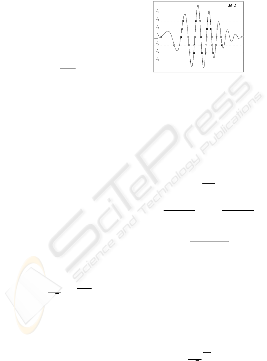
Figure 2: Signal for simplified analysis of SoD sampling
density. The black points are LC samples, while the small
circles are SoD samples.
signal. For the Gaussian process the estimation of
sampling density is not so obvious. To simplify the
analysis, we assume the signal, whose consecutive lo-
cal extremes are with different signs varying around
zero level as shown in Figure 2.
The number of quantization levels is K = 2M+1 with
2M levels placed symmetrically around the zero level.
The number of SoD samples captured can be esti-
mated from the number of LC samples for each quan-
tization level. Obviously for the first level we get
N
SoD
l
1
=
N
LC
l
1
2
. (19)
For the second level we get
N
SoD
l
2
=
N
LC
l
2
−N
LC
l
1
2
+ N
LC
l
1
=
N
LC
l
2
+ N
LC
l
1
2
.
(20)
And similarly for the Mth level we get
N
SoD
l
M
=
N
LC
l
M
+ N
LC
l
M−1
2
. (21)
The number of SoD samples captured on the zero
level equals the number of LC samples on the Mth
level
N
SoD
l
M+1
= N
LC
l
M
. (22)
The total number of SoD samples captured, assuming
that N
SoD
l
m
= N
SoD
l
K+1−m
, is
N
SoD
= 2

N
SoD
l
1
+ ...+ N
SoD
l
M

+ N
SoD
l
M+1
. (23)
From (21), (22) and (23) follows, that
N
SoD
= 2

N
LC
l
1
+ N
LC
l
2
... + N
LC
l
M

(24)
and considering (17) the sampling density is
E[σ
SoD
] =
4f
max
√
3
K−1
2
∑
k=1
e
−
l
2
k
4A
2
f
max
. (25)
SIGNAL-DEPENDENT ANALYSIS OF SIGNALS SAMPLED BY SEND ON DELTA SAMPLING SCHEME
127

3 SIGNAL DEPENDENT
SPECTRUM ANALYSIS
Typically the digital spectral analysis is based on the
transformation of the signal samples set {x(t
n
)} from
time to frequency domain by a set of transformation
functions {W( f,t
n
)}
X( f) =
∑
n
x(t
n
)W( f,t
n
), (26)
For example, the discrete Fourier transform is based
on the set of exponent functions {e
−j2π ft
n
} that are
unrelated to the spectral nature of the signal.
In order to construct signal dependent transforma-
tion functions an approach using Minimum variance
(MV) filter is suggested. The basic idea of the MV
filter is to minimize the variance of the signal on the
output of a selective filter. The frequency response
of such a filter adapts to the spectral components of
the input signal on each frequency of interest (Marple,
1987).
Given the filter coefficients a
1
,a
2
,...,a
p
, the out-
put of the filter at time n is
y
n
=
p
∑
n=1
a
n
x
n−k
= x
T
(n)a, (27)
where x
T
(n) = [x
n
,x
n−1
,...,x
n−p+1
] and
a = [a
1
,a
2
,...,a
p
]
T
. The variance of the output
signal is determined as
ρ = E
n
|y
n
|
2
o
= a
H
Ra, (28)
where R = E

x
∗
(n)x
T
(n)

is the autocorrelation ma-
trix and E {(·)} denotes the expectation operator. The
filter coefficients are found to ensure the sinusoidal
signal with frequency f
0
passes through the filter de-
signed for this frequency without distortion and the
variance (28) for spectral components differing from
f
0
is minimal. The first condition can be written as
p
∑
n=1
a
n
e
−j2π f
0
t
n
= e
H
( f
0
)a = 1, (29)
where e( f
0
) =

e
j2πf
0
t
1
,e
j2πf
0
t
2
,...,e
j2πf
0
t
p

T
. It
means that the gain of the filter response on frequency
f
0
is one. In order to satisfy the second requirement
under condition (29) the coefficients of the MV filter
for the frequency f
0
are determined as (McDonough,
1983):
a
MV
( f
0
) =
R
−1
e( f
0
)
e
H
( f
0
)R
−1
e( f
0
)
. (30)
Inserting (30) into (28) gives the minimum variance:
ρ
MV
=
1
e
H
( f
0
)R
−1
e( f
0
)
. (31)
The value (31) indicates the power of spectral compo-
nents of the input signal at the frequency f
0
.
The proposed approach assumes that frequency
band of spectral analysis is covered by a set of such
MV filters. In general, the frequencies of these fil-
ters can be chosen arbitrarily. The particular case is
if the filter frequencies are located equidistantly and
the frequency step is selected equal to the frequency
step ∆f =
1
Θ
of the Discrete Fourier transform (DFT),
where Θ is observation time of the signal being ana-
lyzed. To obtain a high resolution spectral estimation,
it is reasonable to select the frequency step several
times smaller than the Fourier frequency step.
The expression (31) requires the knowledge of the
signal autocorrelation. The Wiener-Khinchin theorem
relates it to the power spectral density P( f) via the
Fourier transform:
R(τ) =
Z
∞
−∞
P( f)e
j2πfτ
d f (32)
In order to obtain P( f) estimate at the frequencies f =
[ f
1
, f
2
,..., f
M
] from the non-uniformly spaced signal
samples
ˆ
x = [x
1
,x
2
,...,x
N
] the DFT can be used
ˆ
P
(DFT)
=




ˆ
xB
T
N




2
, (33)
where B is M ×N matrix whose element in row m
and column n is b
mn
= e
−j2π f
m
t
n
. The elements of au-
tocorrelation matrix from the spectral estimation can
be calculated on the bases of inverse DFT
ˆr
lk
=
M
∑
m=1
ˆp
(DFT)
m
b
∗
ml
b
mk
. (34)
As the signal autocorrelation matrix (34) is rather
rough estimate then the resulting PSD function values
ˆ
P = [ ˆp
1
, ˆp
2
,..., ˆp
M
], where ˆp
m
= ρ
MV
( f
m
), obtained
by (31)
ˆ
P =
1
diag(BR
−1
B
H
)
(35)
will not provide precise results.
To increase the precision a special iterative algo-
rithm is used (Liepinsh, 1996), (Greitans, 1997) ac-
cording to which the (i+ 1)-th order estimate of sig-
nal autocorrelation matrix is updated from i-th order
ˆ
P
(i)
estimate in the following way
ˆr
(i+1)
lk
=
M
∑
m=1
ˆp
(i)
m
b
∗
ml
b
mk
. (36)
The values
ˆ
P
(i)
are obtained as
ˆ
P
(i)
=





ˆ
xR
(i)
−1
B
H
diag(BR
(i)
−1
B
H
)





2
(37)
SIGMAP 2008 - International Conference on Signal Processing and Multimedia Applications
128

considering that the power of the output of the de-
signed MV filter
p( f
0
) = |
ˆ
xa
MV
( f
0
)|
2
(38)
is interpretable similarly to the power of the output of
selective Fourier filter
p
DFT
( f
0
) = |
ˆ
xe
∗
( f
0
)|
2
(39)
at the frequency f
0
.
The iteration process begins with the initial PSD
values
ˆ
P
(0)
=
ˆ
P
(DFT)
. The iteration process can be
stopped when the difference k
ˆ
P
(i+1)
−
ˆ
P
(i)
k becomes
small.
4 SIMULATION RESULTS
As a test-signal an autoregressive moving-average
(ARMA) process with AR coefficients c(1) = −2.76,
c(2) = 3.809, c(3) = −2.654, c(4) = 0.924 and MA
coefficients d(1) = −0.9, d(2) = 0.81 was used. The
PSD function of such signal is given as (Marple,
1987):
P
ARMA
( f) =
1
2f
max





1+
∑
V
v=1
d(v)e
−jπv f / f
max
1+
∑
U
u=1
c(u)e
−jπu f / f
max





2
,
(40)
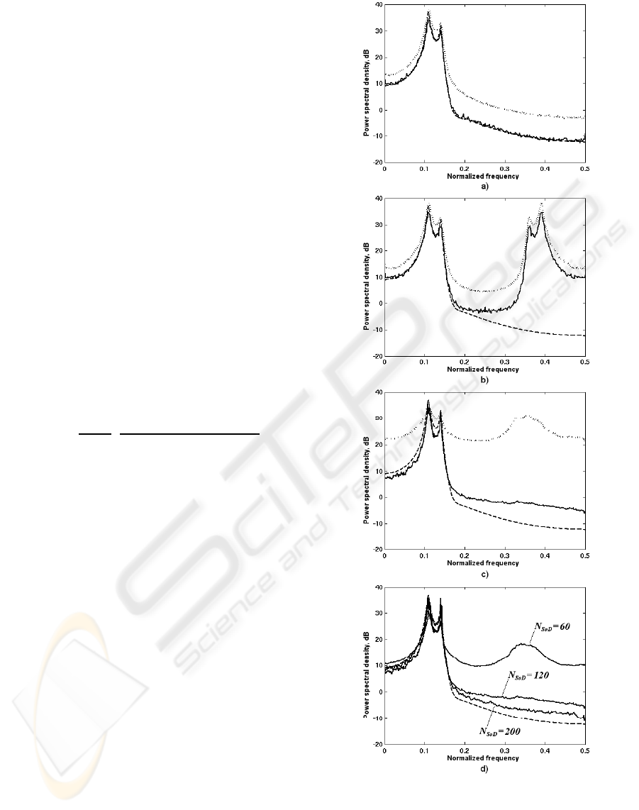
and is shown as a dashed line in Figure 3.
To show the potential of the send-on-delta sam-
pling and performance of proposed signal-dependent
method, the results were compared with uniformly
sampled signal case. The test-signal with f
max
= 0.5
was sampled during 256 seconds and processed with
iterative algorithm described in Section 3. The solid
line in Figure 3a illustrates the PSD estimate if sig-
nal is sampled uniformly at Nyquist rate (256 sam-
ples), while the dotted line shows spectrum estimated
by the standard minimum variance filter (Capon fil-
ter) approach. The plots are the averages of 100 in-
dependent realizations similarly as in (Li and Stoica,
1998). If the sampling rate is reduced two times (128
samples), the frequency aliases appear as shown in
Figure 3b.
In order to obtain SoD samples, the uniformly
sampled signal (at Nyquist rate) was interpolated by
sinc functions. To decrease the interpolation error the
test-signal with duration of 512 seconds was interpo-
lated and thereafter sampled by SoD from 128 to 384
seconds. Figure 3c demonstrates the case, where the
sampling was done using 11 quantization levels. In
total 120 samples (the average number for 100 inde-
pendent realizations) were captured. The dotted line
shows PSD estimate obtained by the expression (35)
Figure 3: PSD estimates using different sampling schemes:
a) uniform at Nyquist rate, b) uniform below Nyquist rate,
c) SoD with 11 levels d) SoD with 7, 11 and 15 levels
(dashed line - true PSD, dotted line - estimate without it-
erations and solid line - estimate after the 10th iteration.
SIGNAL-DEPENDENT ANALYSIS OF SIGNALS SAMPLED BY SEND ON DELTA SAMPLING SCHEME
129

without iterative updating of autocorrelation matrix
R. The frequency aliasing is well observable. The it-
erative procedure improves the result and suppresses
aliasing. It is shown in figure by solid line, which
illustrates PSD obtained after the 10th iteration. Al-
though the estimate is close to true PSD values, it does
not reach the lower power level of -10dB. However,
the estimate is better than the result obtained in uni-
form sampling case at Nyquist rate using the standard
Capon filter approch (see dotted line in Figure 3a).
If the number of SoD quantization levels was in-
creased to fifteen then average 200 samples were cap-
tured. The results after the 10th iteration are illus-
trated in Figure 3d. In this case the PSD estimate gets
closer to the lower power level of true PSD since we
have more data about the signal. In contrast, if the
number of SoD quantization levels was decreased to
seven then average 60 samples were captured and the
precision of PSD estimate got worse.
5 CONCLUSIONS
The use of send-on-delta sampling provides sev-
eral interesting features − the local sampling den-
sity reflects the local properties of the signal, samples
are without quantization errors in amplitude, non-
uniform location of sampling instants allows suppres-
sion of frequency aliasing that leads to the possibility
of processing signals with a reduced sampling den-
sity. As was shown in the paper, in contrast to the
level-crossing sampling, the SoD scheme guarantees
a certain minimal interval between samples, which is
a principal factor for practical implementations. How-
ever it is done at the expenseof decreasing the number
of samples.
To deal with non-uniformity and the reduced den-
sity of sampling flow, it was proposed to use a pro-
cessing method, which is based on signal depen-
dent transformation. The shortage of samples can
be compensated by the iterative update of the estima-
tion of the autocorrelation matrix. Simulation results
show correct spectral estimation even if the sampling
density is decreased several times in relation to the
Nyquist rate. However it is done at the expense of an
increased computation burden, because a linear sys-
tem of equations has to be solved in each iteration.
In fact, the complexity of the data acquisition
phase is transferred to the processing phase. Such
a strategy offers possibilities for distributed wireless
data acquisition in remote sensing systems. The sig-
nal dependent nature of sampling, the decreased num-
ber of samples and the possibility to code data with
one bit using position on time axis allow considerably
diminish the amount of transmitted data.
REFERENCES
Allier, E. and Sicard, G. (2003). A new class of asyn-
chronous a/d converters based on time quantization.
In ASYNC’03, Proc. of International Symposium on
Asynchronous Circuits and Systems.
Greitans, M. (1997). Iterative reconstruction of lost sam-
ples using updating of autocorrelation matrix. In
SampTA’97, Proc. of the International Workshop on
Sampling Theory and Applications.
Greitans, M. (2005). Spectral analysis based on signal
dependent transformation. In SMMSP’05, Proc. of
the 2005 International TICSP Workshop on Spectral
Methods and Multirate Signal Processing.
Greitans, M. (2006). Processing of non-stationary signal
using level-crossing sampling. In SIGMAP’06, Proc.
of the International Conference on Signal Processing
and Multimedia Applications.
Hauck, S. (1995). Asynchronous design methodologies: An
overview. In Proceedings of the IEEE.
Li, H. and Stoica, P. (1998). Capon estimation of covariance
sequences. Circuits, Systems, and Signal Processing,
17(1):29–49.
Liepinsh, V. (1996). An algorithm for estimation of discrete
fourier transform from sparse data. Automatic control
and computer sciences, 29(3):27–41.
Mark, J. W. and Todd, T. D. (1981). A nonuniform sampling
approach to data compression. IEEE Transactions on
Communications, 29(1):24–32.
Marple, S. M. (1987). Digital spectral analysis with appli-
cations. Prentice Hall.
Masry, E. (1978). Alias-free sampling: An alternative con-
ceptualization and its applications. IEEE Transactions
on Information Theory, 24(3):317–324.
McDonough, R. N. (1983). Application of the maximum-
likelihood method and the maximum-entropy method
to array processing. In Nonlinear Methods of Spectral
Analysis.
Miskowicz, M. (2006). Send-on-delta concept: An event-
based data reporting strategy. Sensors, 6(1):49–63.
SIGMAP 2008 - International Conference on Signal Processing and Multimedia Applications
130