EFFICIENT LOCALIZATION SCHEMES IN SENSOR NETWORKS
WITH MALICIOUS NODES
Kaiqi Xiong and David Thuente
Department of Computer Science, North Carolina State University, Raleigh, NC 27695-7534, U.S.A.
Keywords:
Wireless sensor network (WSN), Sensor localization, Vulnerability, and Security.
Abstract:
The accuracy of location information is critical for many applications of wireless sensor networks (WSN),
especially those used in hostile environments where malicious adversaries can be present. It is impractical
to have a GPS device on each sensor in WSN due to costs. Most of the existing location discovery schemes
can only be used in the trusted environment. Recent research has addressed security issues in sensor network
localization but, to the best of our knowledge, none has completely solved the secure localization problem.
In this paper, we propose novel schemes for secure dynamic localization in sensor networks. The proposed
algorithms tolerate up to 50% of beacon nodes being malicious and they have linear computation time with
respect to the number of reference nodes. We have conducted simulations to analyze their performance.
1 INTRODUCTION
Sensor networks may become the next wave of in-
formation technology. Distributed networks of thou-
sands of collaborative sensors promise long-lived and
unattended systems for many monitoring, surveil-
lance and control applications such as health and gas
pipe monitoring and data acquisition in battlefield and
other hazardous environments. Many applications re-
quire knowledge of sensor positions. The location in-
formation may save energy and life, e.g., see (Hu and
Evans, 2004), (Karp and Kung, 2003), and (Mauve
et al., 2001). Secure location discovery for sensor
networks is crucial in a hostile environment. Without
security, sensor locations may be estimated through
compromised nodes. Finding sensor locations is a
challenging problem due to sensor constraints such as
limited energy, computation, and communication.
Due to computation, power, cost, and storage con-
straints of sensor networks, GPS will not usually be
installed on every sensor node. Furthermore, GPS
works only in outdoor unshielded environments (He
et al., 2003) and (Wellenhoff et al., 1997). In re-
cent years, many localization schemes (see (Bahl and
Padmanabhan, 2000), (Liu et al., 2005a), (Mainnwar-
ing et al., 2002), and (Niculescu and Nath, 2001))
have been proposed for sensor networks without de-
pending on expensive GPS devices. Most of these
schemes assume some special nodes, called beacon
nodes, have the capability to know their own location
either through GPS receiversor manual configuration.
Non-beacon sensor nodes can be equipped with rel-
atively cheap measuring devices for signal strength,
directionality, or time of arrival, etc. The non-beacon
nodes can use these measurements and the locations
of two or more beacon nodes to estimate their own lo-
cations. In addition, range-free techniques have also
been proposed to solve for sensor localization prob-
lem (Bulusu et al., 2004) and (He et al., 2003). No
range equipment except for beacon nodes is needed
in these techniques. For example, a sensor node com-
putes its position using hop-counts received from bea-
cons instead of distances. The hop-count is used as
an estimate of sensor’s physical location. Then the
node finds the average distance per hop through the
beacon node’s communication. Moreover, Niculescu
et al. (Niculescu and Nath, 2001) described a sim-
ilar scheme but improved the accuracy of the dis-
tance estimation by using the average hop count of
all the neighbors of a node as a distance estimate.
When three location references are received by a sen-
sor node, triangulation is used to estimate its loca-
tion. If a node receives more than three location refer-
ences from beacons then the least-square optimization
method will be performed to find the location.
Most of the above protocols discussed are vul-
nerable. Security has played an important role in
many sensor networks applications because sensors
are often unattended and easily attacked. An un-
protected sensor node may localize to a wrong posi-
190
Xiong K. and Thuente D. (2008).
EFFICIENT LOCALIZATION SCHEMES IN SENSOR NETWORKS WITH MALICIOUS NODES.
In Proceedings of the International Conference on Security and Cryptography, pages 190-196
DOI: 10.5220/0001927501900196
Copyright
c
 SciTePress

tion through compromised nodes with possible severe
consequences. Secure localization has attracted con-
siderable attention over the last a few years. In this
paper, we propose several methods for secure location
discovery in sensor networks.
The remainder of this paper is organized as fol-
lows. In section 2 we describe several secure sensor
localization methods, including a secure dynamic lo-
calization method. Security analysis for the secure
dynamic localization method is studied in section 3.
Our simulation results are reported in section 4. Re-
lated work is discussed in section 5 and conclusions
are presented in section 6.
2 SECURE SENSOR
LOCALIZATION METHODS
In this section we present several novel approaches
for secure localization in sensor networks. We de-
scribe two naive methods using the concepts of mean
and median values. Then we develop dynamic local-
ization methods to improve the accuracy of location
estimates so these methods become feasible in prac-
tice.
Let (x, y) be the coordinate of node N which wants
to determine its position. Assume there are n beacons
B
i
that know their own positions (x
i
, y
i
) in the sen-
sor network (i = 1, 2,··· , n). Denote by d
i
the mea-
sured distance between (x, y) and (x
i
, y
i
) which may
stem from the differenttypes of measurements such as
signal strength, time of arrival or hop count in a sin-
gle or multi-hop sensor network, see (Bulusu et al.,
2004), (Doherty et al., 2001), (He et al., 2003) and
(Niculescu and Nath, 2001). The problem of secure
sensor localization is to find an accurate location esti-
mation based on references from beacons when there
are malicious beacons.
In this section we present two simple localiza-
tion methods: the mean-based localization method
and the median-based localization methods. How-
ever, a single malicious reference may result in the av-
erage value far from its true coordinate in the former
method. Moreover, the latter method can only toler-
ate up to about 20% malicious beacon reference nodes
(see section 3). Hence, we propose secure localization
schemes and secure dynamic localization schemes to
improve the median-based localization methods.
2.1 The Mean-based Localization
Method
In the beacon-based technique, the problem of sensor
localization discovery is how to determine the coordi-
nate (x, y) based on the positions of beacon nodes B
i
as references. The triangulation process, usually used
in this technique, of determining the coordinate is to
select three measurement tuples from the collection
{(x
i
, y
i
, d
i
)}
i=1,2,···,n
, and solve for (x, y) based on the
the following equations
(x− x
i
j
)
2
+ (y− y
i
j
)
2
= d
2
i
j
for j = 1, 2,3
Denote the solutions by x = x
j
and y = y
j
for j =
1,2,··· ,m, where m is the total number of combi-
nations consisting of three measurement tuples that
can determine the coordinate. Ideally, the tuple ref-
erence values {(x
i
, y
i
, d
i
)}
i=1,2,···,n
are not disrupted
by a malicious node. Let e
j
i
be the estimated differ-
ence between d
i
and the distance computed by each
derived estimation (x
j
, y
j
) to {(x
i
, y
i
)}
i=1,2,···,n
for
j = 1,2,··· ,m.
Their differences are caused by the presence of
measurement noises. Precisely, let
σ
x
=
"
1
m− 1
m
∑
j=1
(x
j
− µ
x
)
2
#
1
2
, σ
y
=
"
1
m− 1
m
∑
j=1
(y
j
− µ
y
)
2
#
1
2
Then the coordinate (x, y) should follow a two-
dimensional uniform (Gaussian) distribution. Its
probability distribution function is given by:
p(x, y) =
1
2πσ
x
σ
y
e
−
1
2

x−µ
x
σ
x

2
+

y−µ
y
σ
y

2

where σ
x
6= 0 and σ
y
6= 0. For notational simplicity,
let η = η(x,y) be defined by η =
q
(
x−µ
x
σ
x
)
2
+ (
y−µ
y
σ
y
)
2
and we give the following definition.
Definition 1: Given a predefined value γ > 0, coor-
dinate (˜x, ˜y) is called a γ-polluted point if η(˜x, ˜y) ≥ γ.
Thus, a mean-based localization method (MALM)
to determine coordinate (x, y) is given as follows.
Algorithm 1.
1. Select every three measurement tuples from
{(x
i
, y
i
, d
i
)}
i=1,2,···,n
and compute (x
j
, y
j
) trian-
gulation method. Let S denote a collection of
(x
j
, y
j
) (j = 1,2,··· ,m).
2. For each (x
j
, y
j
) and a predefined γ (usually γ >
1), determine if (x
j
, y
j
) is a γ-polluted point. If
yes, delete it from S. Repeat the step until all ele-
ments in S are checked. Denote the remaining set
of S by
ˆ
S.
3. Calculate the average point ( ˆx, ˆy) by computing
the average x-coordinate and y-coordinate values
of all elements in
ˆ
S. Then (ˆx, ˆy) is an estimation
coordinate of (x, y) for sensor N.
However, when there are malicious nodes in a sen-
sor network, some of values (x
j
, y
j
) may be signif-
icantly different from the true values because of an
EFFICIENT LOCALIZATION SCHEMES IN SENSOR NETWORKS WITH MALICIOUS NODES
191

attack such as a wormhole attack. When the number
of samples is small, a single incorrect value (x
j
, y
j
)
may significantly change the distribution of (x
j
, y
j
)
( j = 1,2,··· , m). Thus, the MALM method will not
work well. This is because a mean-value point may
not be in the center of measurement tuples. To im-
prove the estimation, we now propose the following
methods based on the concept of a center of gravity.
2.2 The Median-based Localization
Methods
When there is a significant point far away from others,
a mean-value point is not in the center of estimation
points. The median-value point is located in the cen-
ter of these estimation points in term of a predefined
metric and is a random variable (a robust estimator of
the center) (Huber, 1981).
Let d
j
be the Euclidean distance of (x
j
, y
j
)
from the origin given by d
j
=
p
(x
j
)
2
+ (y
j
)
2
( j =
1,2,··· ,m). Sort the sequence {d
j
} ( j = 1, 2, · ·· ,m)
in increasing order. Without loss of generality, as-
sume that the sequence {(x
1
, y
1
),··· ,(x
m
, y
m
)} is
sorted. A simple way to define the center of the
sequence {(x
j
, y
j
)}
j=1,2,···,m
is to use distance d
j
as a measure. The median point of the sequence
{(x
j
, y
j
)}
j=1,2,···,m
is, (x
M
, y
M
) is a point such that
d
M
=
p
(x
M
)
2
+ (y
M
)
2
is in the center of sequence
{d
j
}
j=1,2,···,m
. Then x
M
= x
m+1
2
if m is odd; other-
wise, x
M
=
x
m
2
+x
m
2
+1
2
. Similarly, y
M
is defined. How-
ever, such a definition does not really reflect the cen-
ter of sequence {(x
j
, y
j
)}
j=1,2,···,m
. Here we let x
M
and y
M
be the medians of sequences {x
j
} and {y
j
}
respectively. Then (x
M
, y
M
) is used as the center
of sequence {(x
j
, y
j
)}. Another possible definition
is to use such a point in {(x
j
, y
j
)} (j = 1,2,··· , m)
that it is the closest to (x
M
, y
M
) in term of an Eu-
clidean distance. Please also refer (Bernholt and
Fried, 2003) for a further definition and computa-
tion of a median as well. For the estimation points
(x
j
, y
j
), we can shift them by (x
M
, y
M
), denoted
˘x
j
= x
j
− x
M
and ˘y
j
= y
j
− y
M
. Then we calculate
their means by ˘µ
x
=
1
m
∑
m
j=1
(x
j
− x
M
) = µ
x
− x
M
and
˘µ
y
=
1
m
∑
m
j=1
(y
j
− y
M
) = µ
y
− y
M
. Furthermore, we
compute their standard deviations by
˘
σ
x
=
"
1
m− 1
m
∑
j=1
( ˘x
j
− ˘µ
x
)
2
#
1
2
,
˘
σ
y
=
"
1
m− 1
m
∑
j=1
( ˘y
j
− ˘µ
y
)
2
#
1
2
It is easy to see that
˘
σ
x
= σ
x
and
˘
σ
y
= σ
y
.
Similar to the previous section, a median-based
localization method (MDLM-1) is derived as follows.
Algorithm 2
.
1
. Use Step 1 in the MALM method to find (x
j
, y
j
)
and then compute (˘x
j
, ˘y
j
) (j = 1,2, · · · ,m).
2. For each (˘x
j
, ˘x
j
) and a predefined γ (usually γ >
1), determine if (˘x
j
, ˘x
j
) is a γ-polluted point. If
yes, delete it from S. Repeat the step until all ele-
ments in S are checked and denote the remaining
set of S by
ˆ
S. At this time, note that η is given by
η =
q
(
˘x−˘µ
x
˘
σ
x
)
2
+ (
˘y−˘µ
y
˘
σ
y
)
2
.
3. Calculate the average point by computing the av-
erage values of x-coordinate and y-coordinate of
all elements in
ˆ
S respectively, denoted by ( ˆx, ˆy).
Then ( ˆx, ˆy) is an estimation coordinate of (x, y)
for sensor N.
The difference between MALM and MDLM-1 meth-
ods is that (x
j
, y
j
) is shifted by its mean value in
MALM and its median-valuepoint in MDLM-1. Both
methods have the computation time of Θ(m).
Let e
j
i
be the difference between d
j
and the esti-
mated distance computed by each estimated coordi-
nate (x
e
, y
e
) to {(x
i
, y
i
)}
i=1,2,···,n
for j = 1,2,··· , m.
Assume that e
j
i
follows a normal distribution with
mean value 0 and standard deviation ε. (Note that we
do not care about the specific distribution of e
j
i
. We
only need to have the absolute value of e
j
i
’s offset, de-
noted by the parameter ε.) Then we derive a different
median-based localization method, called MDLM-2.
Algorithm 3
.
1
. Use Step 1 in MALM to find (x
j
, y
j
) and their
median coordinate (x
M
, y
M
) (j = 1,2,··· , m).
2. For each {(x
i
, y
i
)}
i=1,2,···,n
, compute
e
i
= d
i
−
q
(x
i
− x
M
)
2
+ (y
i
− y
M
)
2
Let D be the set of points {(x
i
, y
i
, d
i
)} satisfying
|e
i
| ≤ ε
3. Apply the minimum mean square error (MMSE)
method to D to find an estimation coordinate of
(x, y) for sensor N.
MDLA-2 rechecks the accuracy of (x
M
, y
M
), a predic-
tion by computing e
j
i
. But, (x
M
, y
M
) can be produced
by correct location references only if a sensor network
has no more than 20% malicious beacons. A study is
conducted to verify this in section 3.
2.3 The Secure Dynamic Localization
Method
In the previous two sections, we developed three lo-
calization methods for securely determining the co-
ordinates of a sensor. The efficiency of these three
SECRYPT 2008 - International Conference on Security and Cryptography
192

methods depends on m. Every three nonlinear tuples
{(x
i
, y
i
, d
i
)}
i=1,2,···,n
can be used to derive an estima-
tion coordinate. There are

n
3

possible choices in se-
lecting 3 from n, that is, m =

n
3

=
n(n−1)(n−2)
6
. Re-
call that each of these three previous methods has the
computational cost of Θ(m). For example, when there
are 150 beacons, m = 551300. Hence, all three meth-
ods are computationally burdensome to a sensor with
low computational capacity or depletable battery. We
will present an algorithm that significantly enhances
the efficiency of the MDLM-2 method and also toler-
ates up to 50% beacon nodes being malicious.
We denote by A the collection of measurement
tuples {(x
i
, y
i
, d
i
)}
i=1,2,···,n
. The secure localization
method (SELM) is:
Algorithm 4.
1
. Choose an integer number r and randomly select k
measurement tuples from A . By applying Step 1
in Algorithm 1 to every three of the chosen k mea-
surement tuples, we find its estimated coordinates
and their median coordinate. Repeat the above
procedure r times and let (x
M
j
, y
M
j
) be the median
coordinate where j = 1,··· ,r, and k should be
chosen as 3 ≤ k << n.
2. For each (x
M
j
, y
M
j
), calculate
e
i j
= d
i
−
q
(x
i
− x
M
j
)
2
+ (y
i
− y
M
j
)
2
for i = 1, 2, · · · ,n and j = 1, 2, ··· ,r.
3. For a predefined value ε > 0, let D
j
be a set of
such points {(x
i
, y
i
, d
i
)} satisfying |e
i j
| ≤ ε. Let
D
max
be one of {D
j
}
j=1,2···,r
that contains the
largest number of elements.
4. By applying the MMSE method to D
max
, we find
an estimation coordinate of (x, y) for sensor N.
Clearly, the computation times are Θ(rk
3
) for Step
1, Θ(rn) for Steps 2 and 3, and Θ(|D
max
|) for
Step 4, where |D
max
| is the number of elements in
D
max
. Thus, the total computation time of Algo-
rithm 4 is C=Θ(rk
3
)+Θ(rn)+Θ(|D
max
|). That is, C =
max{Θ(rk
3
), Θ(rn)} is much less than the computa-
tion time, Θ(n
3
), in Algorithms 1-3 respectively since
r can be chosen as a small number. In section 3, we
prove that for a given k, we can get a correct median
coordinate as the estimation of node N’s position in r
times, when r is chosen as a sufficiently big (but still
small) integer. We will show how to choose positive
integers k and r to meet predefined performance based
on affordable resources in section 3. According to our
analysis there, r can be chosen as a relatively small
number and the computation time of Algorithm 4 is
approximately equal to max{Θ(k
3
), Θ(n)}. Further-
more, since more than 50% of beacon nodes provide
correct reference information, D
max
will be generated
by a correct median coordinate that is computed based
on correct location references, or a correct estimation
of node N’s coordinate, according to the computation
method of the median coordinate.
In Algorithm 4, r is a pre-selected value based on
the information provided in the security analysis of
section 3. However, due to the limited computation
and storage in sensor networks, any extra computa-
tion and storage may be a burden and deplete the bat-
tery. Moreover, we may be lucky to get a correct
median coordinate before finishing r rounds. This
suggests the following secure dynamic localization
method (SDLM).
Algorithm 5
.
1
. Randomly select k measurement tuples from A .
By applying Step 1 in Algorithm 1 to every three
of the chosen k measurement tuples, we find its es-
timated coordinates and their median coordinate,
denoted as {(x
M
, y
M
)}, where 3 ≤ k << n.
2. For each (x
M
, y
M
)}, calculate
e
i
= d
i
−
q
(x
i
− x
M
)
2
+ (y
i
− y
M
)
2
(i = 1, · · · , n)
3. For a predefined value ε > 0, let D be a set of such
points {(x
i
, y
i
, d
i
)} satisfying |e
i
| ≤ ε.
4. If D contains more than 50% of beacon nodes,
then apply MMSE to D to find an estimation coor-
dinate of (x, y) for sensor N, denoted by (x
e
, y
e
).
5. For a predefined δ > 0, calculate
ˆe
i
= d
i
−
q
(x
d
i
− x
e
)
2
+ (y
d
i
− y
e
)
2
where (x
d
i
, x
d
i
)∈ D (i = 1, 2,· · · , |D |).
If
1
|D |
∑
|D |
i=1
| ˆe
i
| ≤ δ, then select (x
e
, y
e
) as the
estimation of (x, y) for node N’s coordinate and
then exit. Otherwise, repeat Steps 1-5.
Similarly, the computation times are Θ(k
3
) for Step
1, Θ(n) for Steps 2 and 3, Θ(|D |) for Step 4, and
Θ(|D |) for Step 5. Thus, the total computational cost
of Algorithm 5 is C = Θ(k
3
) + Θ(n) + Θ(|D |) multi-
plied by the number of repeated times. As mentioned
early, the number of repeated times is usually small
as studied in section 3. Hence, the computational
cost in Algorithm 5 is max{Θ(k
3
), Θ(n)}. Hence, Al-
gorithm 5 also has much less computation time than
Algorithms 1-3. Accordingly, the selection of δ > 0
is based on a sensor’s performance requirement and
available resources. Usually, δ > 0 should be cho-
sen as a value such that it is bigger than ε > 0. This
is because using the MMSE method to find a best-
fit cannot guarantee that it satisfies |e
i
| ≤ ε for all
EFFICIENT LOCALIZATION SCHEMES IN SENSOR NETWORKS WITH MALICIOUS NODES
193

(x
d
i
, x
d
i
)∈ D (i = 1, 2,··· ,|D |). Moreover, from the
above analysis we know that if the number of itera-
tions in Algorithm 5 is big enough, such a coordinate
(x
e
, y
e
) can be found.
Algorithms 4 and 5 greatly improve the efficiency
of MDLM-1 and MDLM-2. The SDLM method can-
not guarantee deriving an optimal coordinate of a sen-
sor. But, its solution is sub-optimal. Moreover, an
obvious question is how to choose k. In general, the
smaller k, the less computation time. In particular,
if k is chosen as a number with k ≤ n
1/3
, then the
computation time of the SELM and SDLM methods
is Θ(n), i.e., the SELM and SDLM methods are linear.
To keep SELM and SDLM being practical, k should
be chosen as an integer with k << n. Actually, based
on the security analysis of section 3, k and r can be
chosen as relatively small values.
3 SECURITY PERFORMANCE
ANALYSIS
Algorithms 4-5 are designed based on the same tech-
nique: randomly select k references from n beacons.
Hence, we now only discuss the security performance
analysis of Algorithms 4-5; that is, we seek an r in
Algorithm 4, or the number of repeated times in Al-
gorithm 5 (for simplicity, it is also denoted as r), re-
quired to obtain at least a correct median coordinate
with a given probability so that the location of a sen-
sor can be closely estimated.
Recall that n represents the number of beacon
nodes in a sensor network that can provide location
references for node N. Let q be the number of ma-
licious nodes among these beacon nodes in the net-
work. In the first round of the SELM method, we ran-
domly select k measurement tuples in A from n bea-
con nodes, and then estimate the coordinate of node
N by every three tuples chosen from the k nodes. The
total number of estimated coordinates is

k
3

.
Let’s first study how by chance we can get over
50% coordinates that are not determine by any sin-
gle malicious nodes in the chosen k beacons. De-
note by b the malicious nodes in the chosen k bea-
cons. Then, the probability that a coordinate is not
determined by malicious beacons is p
b
=
(
k−b
3
)
(
k
3
)
=
(k−b)(k−b−1)(k−b−2)
k(k−1)(k−2)
. By using both analytical and
simulation methods, we have found that in order to get
p
b
≥ 50%, we need to approximately have b ≤ ⌊
k
5
⌋,
that is, no more than 20% of the chosen k beacons
are malicious, where ⌊
k
5
⌋ is a floor value of
k
5
. (Note
that the analysis also indicates that Algorithms 1 and 2
Table 1: The number of repeated times so that 99% chance
to obtain at least one correct median coordinate.
Percentage of Malicious Location References
30% 40% 50%
k=5 r=6 r=11 r=21
k=10 r=12 r=25 r=84
can only tolerate up to about 20% beacon nodes being
malicious.) In the first round, the probability for se-
lecting exactlyt measurement tuples from q malicious
nodes is p(t) =
(
q
t
)(
n−q
k−t
)
(
n
k
)
. As is known, we can deter-
mine the coordinate of node N correctly if less than
half of these k nodes are malicious. Consequently,
the probability that we can determine coordinates for
node N is
p =
⌊
k
5
⌋
∑
t=0
p(t) =
⌊
k
5
⌋
∑
t=0

q
t

n−q
k−t


n
k

Note the identity
∑
k
t=0

q
t

n−q
k−t

=

n
k

.
We want the probability that we randomly se-
lect k reference tuples from n beacon nodes and re-
peat the selection r times. Then, the probability that
we have at least one chance to get a median coordi-
nate as a correct estimation of node N’s coordinate
is P = 1 − (1 − p)
r
. Table 1 shows the number of
times (r) that we need to repeatedly choose (k) loca-
tion references so that we have 99% chance to get at
least one correct median coordinate in r trials, when
k=5 and 10. Subsequently, we can find D
max
in Algo-
rithm 4 and the estimated coordinate of sensor node
N when ε > 0 is properly chosen. Surprisingly, when
p is fixed, the selection of k and r does not depend on
the number of beacon nodes, n, based on our simula-
tion. Also, the chance that we can get a correct me-
dian does not increase as k increases. Conversely, the
bigger k, the bigger r. This means that the more com-
putation and storage cost is required as k increases.
Hence, according to our experiment, k = 5 is a good
selection.
Due to the above analysis, k and r can be chosen
as very small integers compared to n. Hence, Algo-
rithms 4-5 usually have linear computation time with
respect to the number of beacon nodes n. However,
Algorithms 1-3 have cubic computation time in n.
4 NUMERICAL SIMULATION
In this section we shall demonstrate the simulation re-
sults of our proposed method. Due to the page limit
we only present the simulation results of Algorithm 5
in section 2.3. We shall show how the SDLM method
performs in terms of localization error and efficiency.
SECRYPT 2008 - International Conference on Security and Cryptography
194

In the simulation, we assume that all beacon nodes
including malicious nodes are evenly deployed in an
200× 200m
2
square field. Assume that a non-beacon
node can receive the signal from each beacon node in
this field, but a certain percentage of beacon nodes de-
clare their wrong location information due to attacks.
We implement SDLM in Java program over a Linux
environment. We assume the origin point in the co-
ordinate system as the true location of a sensor that
we want to find. A set of 500 beacon references are
first randomly created. Each point contains a tuple of
(x, y, d). d is the distance from the reference point to
the origin. These references may be malicious points.
Value d may be incorrect because of incorrect val-
ues x and y, where d is calculated by d =
p
x
2
+ y
2
.
We assume a simple measurement error model, i.e.,
each sensor cannot be further away from its true loca-
tion by more than 4 meters. That is, ε in the SDLM
method is chosen as 4 meters. This is used to elimi-
nate malicious references. In each run, we randomly
choose 10 references from the 500 beacon references,
i.e., k = 10. The number of runs is 20.
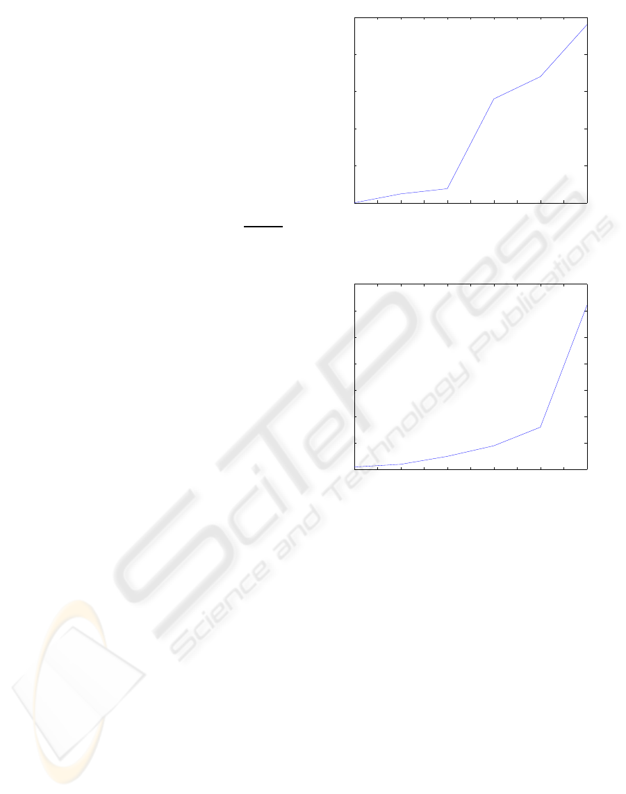
We measured the localization error as the distance
from the estimated location to the true location which
is the origin. It is shown in Figure 1 that the distance
error increases as the percentage of malicious nodes
around the sensor node’s location to be estimated in-
creases. We can see that the error is below 3 meters
even when 50% of reference nodes are malicious. In
most applications, that distance error may be accept-
able. For example, such applications include finding
a missing child in a forest or identifying the location
of natural disaster. In applications which have a high
demand on location information such as routing pro-
tocols, our algorithm can be still used if the number
of malicious nodes is less than 10% percent of all ref-
erence nodes in the non-polluted range.
Furthermore, we study the efficiency of the
method compared to the percentage of malicious
nodes. In the simulation, we use k = 10 and define the
efficiency as the number of runs required to find the
accurate location. This test is performed by a brute
force method. From Figure 2, we see that a sensor
can find its location in fewer steps than the number
of steps based on our analytic model, presented in Ta-
ble 1 when the percentage of malicious nodes is 30%,
40% and 50%.
5 RELATED WORK
Many studies have been conducted on secure loca-
tion discovery for wireless sensor networks in the last
a few years, for example, (Bahl and Padmanabhan,
0 5 10 15 20 25 30 35 40 45 50
0
0.5
1
1.5
2
2.5
The Percentage of Malicious Nodes %
The Distance Estimation Error of Sensor’s Location
The Distance Estimation Error of Sensor’s Location vs. The Percentage of Malicious Nodes
Figure 1: The Distance Estimation Error of Sensor’s Loca-
tion. The Unit of y Axis is Meter.
0 5 10 15 20 25 30 35 40 45 50
0
10
20
30
40
50
60
70
The Percentage of Maliciou Nodes %
The Number of Runs Required to Obtain The Estimation of Sensor’s Location
The Number of Runs Required to Obtain The Estimation of Sensor’s Location vs. The Percentage of
Malicious Nodes
Figure 2: The Number of Runs Required to Obtain The Es-
timation of Sensor’s Location.
2000), (Liu et al., 2005a), (Mainnwaring et al., 2002),
and (Niculescu and Nath, 2001). In this section, we
summarize related work.
Time of arrival (TOA) technology is commonly
used as a means of obtaining range information via
signal propagation time (He et al., 2003). It is
used in GPS for the most basic localization system
(Wellenhoff et al., 1997). However, GPS is expensive
for sensor networks. The time difference of arrival
(TDOA) technique for range estimation between two
communication nodes has been widely proposed as
a necessary ingredient in sensor localization. Many
infrastructure-based systems have used TDOA as a
range estimating tool, for example, see (Bahl and
Padmanabhan, 2000), (Doherty et al., 2001), (Priyan-
tha et al., 2000) and (Want et al., 1992). Doherty,
et al. in (Doherty et al., 2001) formulated the lo-
calization problem as a convex optimization problem
and then solved it using the convex optimization ap-
proach. In (Bahl and Padmanabhan, 2000), received
signal strength indicator (RSSI) was used to translate
EFFICIENT LOCALIZATION SCHEMES IN SENSOR NETWORKS WITH MALICIOUS NODES
195

signal strength into distance estimates.
In addition, range-free techniques have also been
proposed to solve for sensor localization problem (see
(Bulusu et al., 2004), (He et al., 2003), and (Niculescu
and Nath, 2001)). The centroid of all locations in the
received beacon signals has been proposed for sen-
sor’s location discovery in (Bulusu et al., 2004). In
(Niculescu and Nath, 2001) DV-hop was used as an
alternative solution. A sensor node computes its posi-
tion using hop-counts received from beacons, instead
of distances. Then, the node finds the average dis-
tance per hop through beacon nodes’ communication.
The range-based localization schemes have been
enhanced to address security concerns for sensor
networks (e.g., (Liu et al., 2005a) and (Liu et al.,
2005b)). Both an attack-assistant MMSE-based loca-
tion estimation and a voting-based location estimation
have been proposed to deal with attacks in location
discovery in (Liu et al., 2005a). In the first method,
the key point is to find a consistency set. That is usu-
ally not an easy task. There is the same difficulty
seeking the highest vote area as in the latter method.
Furthermore, in (Liu et al., 2005b) Liu et al. provided
a method to reason about the suspiciousness of each
beacon node at the base station based on the detec-
tion information from beacon nodes. In (Fretzagias
and Papadopouli, 2004), Fretzagias et al. proposed
another voting-based scheme, called the Cooperative
Location Sensing (LCS).
Our median-based method is inspired by the cen-
troid technique (Bulusu et al., 2004) and the MMSE
method. As indicated, a mean value does not reflect
the center of location references. Instead, a median
is used to filter out outliers. In this paper we pro-
pose new median-based schemes for dealing with ma-
licious references. In Algorithms 4-5 we can easily
filter out malicious references and then estimate the
location of a sensor node by using the MMSE method.
6 CONCLUSIONS
In this paper we proposed a suite of secure local-
ization methods, including the secure dynamic local-
ization method (Algorithm 5), for sensor networks.
A median-based technique instead of a mean-based
technique was used to represent the center of loca-
tion references so that malicious reference informa-
tion could be filtered out easily. Our security perfor-
mance analysis has shown that the proposed secure
localization methods can tolerate up to 50%malicious
beacon nodes, and they usually have linear computa-
tion time. This is the best we can achieve. We further
conducted simulations to demonstrate the applicabil-
ity and accuracy of these algorithms. Preliminary val-
idation tests showed that Algorithms 4-5 have a good
accuracy against other algorithms. Detailed valida-
tion results are not provided due to the page limit.
REFERENCES
Bahl, P. and Padmanabhan, V. (2000). An in-building RF-
based user location and tracking system. In Proceed-
ings of the IEEE INFOCOM ’00.
Bernholt, T. and Fried, R. (2003). Computing the update
of the repeated median regression line in linear time.
Information Processing Letters, (88):111–117.
Bulusu, N., Heidemann, J., and Estrin, D. (2004). GPS-less
low cost outdoor localization for very small devices.
IEEE Personal Communications Magazine, 7(5):28–
34.
Doherty, L., Pister, K., and Ghaoui, L. (2001). Convex opti-
mization methods for sensor node position estimation.
In Proceedings of INFOCOM ’01.
Fretzagias, C. and Papadopouli, M. (2004). Cooperative
location-sensing for wireless networks. In Proceed-
ings of IEEE PerCom ’04.
He, T., Huang, C., Blum, B. M., Stankovic, J., and Ab-
delzaher, T. (2003). Range-free localization schemes
for large scale sensor networks. In MobiCom ’03.
Hu, L. and Evans, D. (2004). Localization for mobile sensor
networks. In MobiCom ’04.
Huber, P. J. (1981). Robust statistics. Addison-Wesley Pub-
lishing Company, New York.
Karp, B. and Kung, H. (2003). Greedy perimeter stateless
routing. In MobiCom’03.
Liu, D., Ning, P., and Du, W. (2005a). Attack-resistant lo-
cation estimation in sensor networks. In Proceedings
of IPSN ’05.
Liu, D., Ning, P., and Du, W. (2005b). Detecting malicious
beacon nodes for secure location discovery in wireless
sensor networks. In Proceedings of IPSN ’05.
Mainnwaring, A., Polastre, J., Szewczyk, R., Culler, D.,
and Anderson, J. (2002). Wireless sensor network for
habitat monitoring. In Proceedings of ACM WSNA’02.
Mauve, M., Widmer, J., and hartenstein, H. (2001). A sur-
vey on position-based routing in mobile Ad-Hoc net-
works. IEEE Network Magazine.
Niculescu, D. and Nath, B. (2001). Ad hoc positioning sys-
tem (APS). In Proceedings of IEEE GLOBECOM ’01.
Priyantha, N., Chakraborty, A., and Balakrishnan, H.
(2000). The cricket location-support system. In Pro-
ceedings of MOBICOM ’00.
Want, R., Hopper, A., Falcao, V., and Gibbons, J. (1992).
The active badge location systems. ACM Transactions
on Information Systems.
Wellenhoff, H., Lichtenegger, H., and Collins, J. (1997).
Global Positions System: Theory and Practice, Fourth
Edition. Springer Verlag.
SECRYPT 2008 - International Conference on Security and Cryptography
196