EFFICIENT SUPPORT COUNTING OF CANDIDATE ITEMSETS

FOR ASSOCIATION RULE MINING

Li-Xuan Lin, Don-Lin Yang, Chia-Han Yang

Dept. of Information Engineering and Computer Science, Feng Chia University, Taiwan

Jungpin Wu

Dept. of Statistics and Dept. of Public Finance, Feng Chia University, Taiwan

Keywords: Association rules, frequent itemsets, distributed data mining, incremental.

Abstract: Association rule mining has gathered great attention in recent years due to its broad applications. Some

influential algorithms have been developed in two categories: (1) candidate-generation-and-test approach

such as Apriori, (2) pattern-growth approach such as FP-growth. However, they all suffer from the

problems of multiple database scans and setting minimum support threshold to prune infrequent candidates

for process efficiency. Reading the database multiple times is a critical problem for distributed data mining.

Although more new methods are proposed, like the FSE algorithm that still has the problem of taking too

much space. We propose an efficient approach by using a transformation method to perform support count

of candidate itemsets. We record all the itemsets which appear at least one time in the transaction database.

Thus users do not need to determine the minimum support in advance. Our approach can reach the same

goal as the FSE algorithm does with better space utilization. The experiments show that our approach is

effective and efficient on various datasets.

1 INTRODUCTION

Association rule mining (Wang, 2005) has been

widely used in the applications of bioinformatics,

medical diagnosis, Web mining, and various data

analysis. Association rules represent the relationship

between attributes in the form of rules that can

enhance the understanding and application of the

underlying information for users.

In traditional methods, the minimum support is a

very important segment in association rule mining.

The association rules are generated by using the

minimum support. If the minimum support is set too

high, we may lose some useful information. If the

minimum support is too low, we may produce some

useless information. How to determine a good

minimum support is a very important subject. We

want to develop a novel approach which can

efficiently mine association rules without the need of

predetermining the minimum support threshold from

transaction databases.

Some influential algorithms have been

developed in two categories (Hipp, 2000): (1)

candidate-generation-and-test approach such as the

Apriori (Agrawal, 1994) and GSP (

Srikant, 1996), (2)

pattern-growth approach such as the FP-growth

(Han, 2000) and PrefixSpan (Pei, 2004). However,

they all suffer from the problem of multiple database

scans and setting minimum support thresholds to

prune infrequent candidates for process efficiency

and obtaining useful associate rules with support

counts above the threshold value.

To remedy the above problems, our approach has

the following characteristics:

1. No multiple database scans.

2. No need to use previously found frequent

itemsets for candidate generation when we can

directly enumerate all candidate items with

non-zero count.

3. No predetermination of minimum support.

In this approach, we can get all the information

of items from the database. Afterwards, users can set

the best minimum support after they decide what

they want.

180

Lin L., Yang D., Yang C. and Wu J. (2008).

EFFICIENT SUPPORT COUNTING OF CANDIDATE ITEMSETS FOR ASSOCIATION RULE MINING.

In Proceedings of the Third International Conference on Software and Data Technologies - ISDM/ABF, pages 180-185

DOI: 10.5220/0001888101800185

 SciTePress

2 RELATED WORK

To alleviate the problems mentioned in the last

section, some new methods are devised using

different approaches. In the following, we examine

two algorithms belonging to these new approaches,

on which our proposed algorithm is based.

2.1 Fast Support Enumeration

Algorithm: FSE

To generate association rules without the condition

of predetermining the minimum support threshold,

one scan the transaction database once and

enumerate all candidate itemsets with efficient

indexing of their support counters. Thus, it can

produce meaningful rules very easily for any item

that appears at least once in the transactions.

The FSE algorithm (Lin, 2006) is such an

approach that has the following five steps:

Step 1: Read a transaction T from the

transaction database D at a time. Here, each item is

identified with the encoded number.

Step 2: Enumerate all candidate n-itemsets X

for the items in each transaction T of the length n.

There is no need to set the minimum support

threshold in this step.

Step 3: Use Pascal triangle to compute the

indexes of support counters for the generated n-

itemsets X and increase the value of their

corresponding counters. The counters are stored

sequentially in n sub-lists where each i-itemset has

one sub-list, i = 1 to n. Note that each counter must

have a non-zero value since every candidate itemset

is generated after examining actual transactions.

This method is different from joining (i-1)-itemsets

to get i-itemsets where i > 1.

Step 4: Repeat the above three steps until the

last transaction is done.

Step 5: When the minimum support is decided,

one can easily visit the list of support counters to

find all frequent itemsets and generate

corresponding rules as needed.

The FSE algorithm attempts to solve the

problems we have discussed previously. However, it

also has some problems of its own. FSE has a good

performance when the length of the candidate

itemset is short. However, it will incur a very high

cost of storage space when the length of the

candidate itemset is long.

2.2 Item-Transformation Approach

The Item-Transformation algorithm (Chu, 2005) is a

novel and simple method that does not belong to the

candidate generation-and-test approach and the

pattern growth approach. It treats the transaction

database as a data stream and finds the frequent

patterns by scanning the database only once. Two

versions of the approach are provided, Mapping-

table and Transformation-function.

Every item in a transaction can be combined

with each other to get all the possible sub-itemsets.

For example, transaction {a, b, c} can generate all

the sub-itemsets {a, b, c, ab, ac, bc, abc}. In the

following, two versions of the Item-Transformation

approach are introduced.

(1) Mapping-table approach: it uses a table to

represent all the sub-itemsets in the transaction by

using bit-map. Taking a 3-item transaction for

example, Table 1 shows all of their sub-itemsets

with a bit map approach.

(2) Transformation-function approach: it uses

a transformation function to achieve the same goal.

The following rules are used to get the Pattern

Vector (PV) inductively. Some pattern vectors are

shown in the last column of Table 1.

Rule 1: The rightmost position of the PV is

always equal to “1”.

Rule 2: If the next position of the Transaction

Vector (TV) has no item, it fills the PV with a “0” in

the corresponding positions. Some transaction

vectors are shown in the second column of Table 1.

Rule 3: If the next position of TV has an item,

it sets the PV with the value(s) of the previous part.

Table 1: A corresponding mapping table for 3 items.

Item

sets

Transaction

Vector

Set of patterns

(- denotes null)

Pattern

Vector

- 000 0000000,- 0000000

a 001 000000,a,- 0000001

011 0000,b,ba,a,- 0000111

b 010 0000,b,0,0,- 0000100

110 c,0,0,cb,b,0,0,- 1001100

111 c,ca,cba,cb,b,ba,a,- 1111111

3 OUR PROPOSED METHOD

Based on the last two approaches in Section 2, we

take the advantage of candidate enumeration and

encoding scheme respectively to develop our

algorithm with the following five steps:

EFFICIENT SUPPORT COUNTING OF CANDIDATE ITEMSETS FOR ASSOCIATION RULE MINING

181

Step 1: Read one transaction from the

transaction database at a time, and use Arabic

numerals starting from one to encode all the items in

the transaction if they are not already numbered in

the previous transaction. From here on, each item is

identified with an encoded number.

Step 2: Enumerate all candidate n-itemsets for

the items in each transaction of the length n. Here n

is the number of distinct items in the transaction. No

minimum support is required here.

Step 3: Use our transformation approach to

transform these candidate n-itemsets to a form of

(X.Y) where X and Y are numerals. Then add each

of them to a new database if it appears the first time.

Step 4: Repeat the above three steps until the

last transaction is processed.

Step 5: When a threshold value of the

minimum support is specified, one can easily visit

the list of support counters to find all frequent

itemsets and generate corresponding rules as needed.

Since the value of the minimum support is a

given threshold value and the process of rule

generation is trivial, we will only describe the

candidate enumeration and support counting part of

our approach in the rest of the paper.

3.1 Main Concept

To meet the requirement of only one database scan

in our approach, we need to generate all possible

candidate n-itemsets after reading each transaction

t={i

,..,i

} from a database D={i

,..,i

}. Here

1≦n≦m and n becomes the maximum length of the

transactions in D at the end of database scan.

Without pre-determining the minimum support, our

approach generates every possible candidate n-

itemsets from all the transaction items. And there is

no need to specify the minimum support in our

candidate generation approach.

Although some (infrequent) itemsets cannot be

pruned during candidate generation, our method

requires only one database scan and allows users to

find association rules satisfying any non-zero

support count. Our challenge has twofold:

1. Find an effective way to enumerate all

possible candidate n-itemsets for each input

transaction. Next, the support count of each

n-itemset is recorded and then retrieved

efficiently later on for frequent itemset

verification to generate interesting rules.

2. Use the most efficient data structure and

indexes to store and access these support

counters.

3.2 Bit Map and Item-Transformation

We adapt the bit map (Dunkel, 1999) approach to

express each transaction in the database. In every

transaction, if an item appears, its corresponding

position (from left to right) will be marked as “1”,

otherwise it is encoded as “0.” Then, we transform

the binary coding system into decimal coding

system.

To illustrate the process, an item showing in the

first position will be displayed as 2

and the second

will be 2

, the n-th item is 2

n-1

and so on. Under this

mechanism, we can transform each of the items into

a decimal number and sum up their decimal values

for the itemset. For example, we assume a

transaction includes two items A and C. By using

the transformation approach we can obtain a bit map

of 101 and a decimal number of 1×2

+0×2

+1×

=1+0+4=5. It is a step by step transformation.

Different items will be transformed into different

numbers. The number is unique for every itemset.

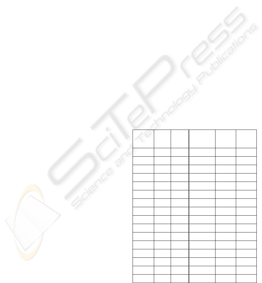
Table 2 shows all the bit map expressions for

items A, B, C, and D in the order of the decimal

system, i.e., decimal numbers from 1 to 31. In Table

2, there are 31 sub-itemsets generated from the

itemset ABCDE. This is the one-dimension case

where a linear expression is used.

Table 2: A mapping table from binary to decimal.

Item

sets

Bit

map

Deci

-mal

value

Item

sets

Bit

map

Deci

-mal

value

A 1 1 E 00001 16

B 01 2 AE 10001 17

AB 11 3 BE 01001 18

C 001 4 ABE 11001 19

AC 101 5 CE 00101 20

BC 011 6 ACE 10101 21

ABC 111 7 BCE 01101 22

D 0001 8 ABCE 11101 23

AD 1001 9 DE 00011 24

BD 0101 10 ADE 10011 25

ABD 1101 11 BDE 01011 26

CD 0011 12 ABDE 11011 27

ACD 1011 13 CDE 00111 28

BCD 0111 14 ACDE 10111 29

ABCD 1111 15 BCDE 01111 30

ABCDE 11111 31

In the two-dimension case, each row can have 2

itemsets. Choosing a proper n=2, it becomes a two-

ICSOFT 2008 - International Conference on Software and Data Technologies

182

dimension array consisting of 4 itemsets in each

row. If n=3, each row will have 8 itemsets. The

itemsets are placed from left to right and from top to

bottom. The first itemset in each row and column is

called the leading itemset. Otherwise, it is called a

non-leading itemset. The only exception is the upper

leftmost entry 0(0) which is treated as null. For

example, A(1) is the leading itemset of the second

column and D(8) is the leading itemset of the third

row. The number in the parentheses is the

corresponding decimal number of the itemset. The

value of n can be defined by the user. Table 3 shows

the result of transforming the representation from

one-dimension to two-dimension.

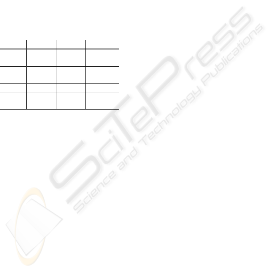
Table 3: A two-dimension list of itemsets.

0(0) A(1) B(2) AB(3)

C(4) AC(5) BC(6) ABC(7)

D(8) AD(9) BD(10) ABD(11)

CD(12) ACD(13) BCD(14) ABCD(15)

E(16) AE(17) BE(18) ABE(19)

CE(20) ACE(21) BCE(22) ABCE(23)

DE(24) ADE(25) BDE(26) ABDE(27)

CDE(28) ACDE(29) BCDE(30) ABCDE(31)

In Table 3 we can observe that each non-leading

itemset is composed of leading itemsets from its

corresponding row and column. Take itemset BCE

for example, it is a combination of the leading

column itemset B and the leading row itemset CE.

The other non-leading itemsets can be verified in the

same way easily. This is a case when the length of

the row or column is 2

The reason for the case of the length 2

is due to

the use of bit map and the binary system. We can

find that after we present the itemsets with bit map

and the row has the length of 2

, the first row

contains a null and the first n items along with their

combinations. And the first column contains a null

and the remaining items along with their

combinations. For n = 2, we can see that the first

row contains the leading itemsets of the first n items

A and B. And the first column contains the leading

itemsets of the rest of items C, D, and E.

Another interesting characteristic of Table 3 is

that the items in the first column can be added

incrementally along with the composed itemsets to

become the leading itemsets. While adding a new

item, it will append its combinations with the

previous results at the end of the table.

For example, the upper half of Table 3 is the list

of itemsets for items {A, B, C, D} in a two-

dimension representation. The corresponding

decimal numbers are from 0 to 15. When we add a

new item E, it will combine with the existing

itemsets of {A, B, C, D} and form the lower part of

Table 3. The corresponding decimal numbers are

from 16 to 31. The newly formed table with the

decimal numbers from 0 to 31 is exactly the same as

Table 3 for itemsets {A, B, C, D, E}. This means

that we can deal with item updates in our approach.

To simply our process, each itemset will be

represented by its corresponding column and row.

We denote their decimal values as X and Y

respectively. Take ABCE (23) for instance, it can be

taken apart as ABCE (23) = AB (3) + CE (20). Here

X = 3 and Y = 20. This indicates that we can

decompose ABCE and obtain a unique

representation of X-column and Y-row.

Our item-transformation method uses the above

concept. In the first step, we define the value of n.

For a two-dimension representation, the length of

the row is 2

. Therefore, the first n items and their

combined itemsets will be placed in the first row

where the remaining items and their combined

itemsets will be placed in the first column in an

ascending order. After we transform the itemsets by

using bit map, their decimal values can be calculated

easily. The first position means 2

, the second

position means 2

, and the n-th position means 2

n-1

To further simply the representation of an itemset in

the two-dimension table with the index of column

and row, we can separate the itemset into two

independent parts (X.Y) where X and Y start from

the origin. Take itemset ABCE as an example, with

n = 2, we can separate the itemset into two parts

which are AB and CE. For sub-itemset AB, we can

get the bit map of 11 and X=1×2

+1×2

=1+2=3. For

sub-itemset CE, we can get the bit map of 101 and

Y=1×2

+0×2

+1×2

=1+0+4=5. Therefore the

itemset ABCE can be transformed into another form

of (X.Y) = (3.5). To verify with Table 3, the itemset

ABCE is composed of the third column and the fifth

row. This indicates that each itemset can be

represented by a unique identifier.

3.3 Support Counting after

Item-Transformation

The next step is to process the transformed sub-

itemsets in the form of (X.Y). We add a third

variable of alphabet “Z” to represent the value of

support counting. The expression of an itemset

becomes (X.Y.Z). The value of Z is initialized to

zero. For better storage management, we sort the

itemsets according to their support count Z first and

then X.Y in ascending order. For updates of adding

additional item, we have the following two cases:

EFFICIENT SUPPORT COUNTING OF CANDIDATE ITEMSETS FOR ASSOCIATION RULE MINING

183

Case 1: Adding a brand new sub-itemset.

Insert the sub-itemset into its corresponding

position in the group of one support count with the

index of (X.Y).

Case 2: Adding an existing sub-itemset.

Increase the sub-itemset’s Z value by one and

move it to the corresponding position in the group of

new Z support count with the index (X.Y).

4 EXPERIMENTAL RESULTS

We performed extensive experiments to compare the

performance of our approach with that of Item-

Transformation, FSE, Apriori, and FP-growth.

4.1 Experimental Environment

We have implemented our algorithm in Java. All the

experiments are performed on a 3.6GHz Intel

Pentium 4 PC machine with 2GB DDR400MHz

memory, running on Microsoft Windows XP with

SP2. We use Java with JDK 1.50 for programming

and eclipse is used as a development tool to build

our experimental environment.

We downloaded existing tools from the ARtool

(Cristoforr, 1999), which has a collection of

algorithms and tools for mining association rules in

binary databases. Note that we use the term “run

time” to show the total execution time (i.e., the

period between input and output), instead of the

CPU time measured in the experiments of some

other literature.

The synthetic datasets which we used for our

experiments were generated from the IBM synthetic

data generator (IBM, 2006). Different sets of

parameters are used to generate various datasets for

performance evaluation. The parameters include the

umber of transactions D, the average size of transactions

T, the average size of maximal potentially–frequent

itemsets I, the number of potentially-frequent itemsets L,

and the number of items N

4.2 Comparison Results

We use the dataset T10I4D0.1K to compare the

performance of our approach with FSE, Apriori and

FP-growth algorithms.

To have a more comparative result for our

experiments, we generate the datasets having the

same number of items N=20. Then we set T=10, I=

4, and L=1000.

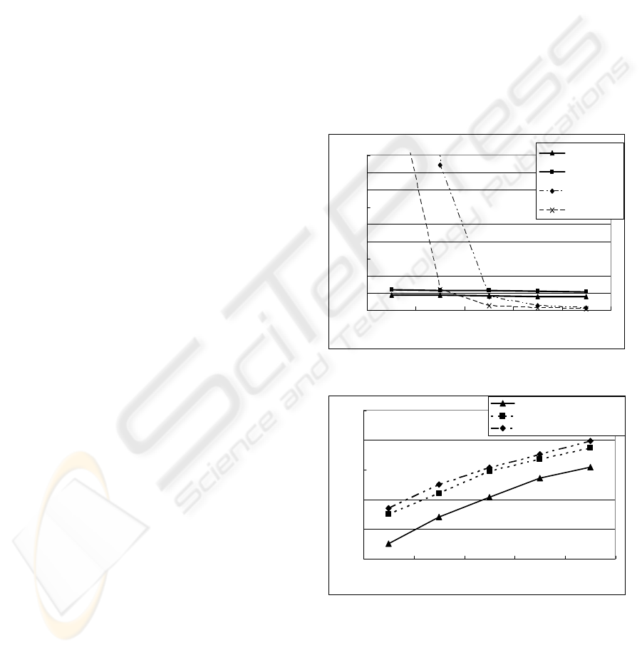
The result of scalability test is shown in Figure 1.

The performance of our algorithm and FSE does not

have any noticeable changes as the minimum

support decreases from 5% to 1% whereas our

approach always runs faster than FSE. Figure 1 also

shows that the performance of FP-growth and

Apriori is better when the support threshold is

greater than 2% and 3% respectively. The reason is

that we did not apply the minimum support

threshold in FSE and our algorithm since we

generate all itemsets with non-zero support counts.

On the other hand, Apriori and FP-growth are not

able to deal with the thresholds smaller than 2% and

1% respectively.

In Figure 2, we use a database which has the

transactions with more repeated items. We can find

that our approach takes less space. It is because that

FSE and Item-Transformation approach reserve the

space for the itemsets that do not appear at that time

but could show up in the later process. So they

would take up more space.

T10.I4.D0.1K

12345

Support threshold(%)

Runtime(sec)

Our approach

FSE

Apriori

gorwth

Figure 1: Scalability test for various min_sup thresholds.

100

150

200

250

100 200 300 400 500

Number of transactions

Space(K .B.)

Our approach

FSE

Item-Transformation A

roach

Figure 2: Space test for different number of transactions.

In Figure 3, it shows that Item-Transformation

approach can deal with the length of transaction less

than 20 and FSE can deal with the length of

transaction less than 25. Our approach can deal with

longer length of transactions with less time. Since

ICSOFT 2008 - International Conference on Software and Data Technologies

184

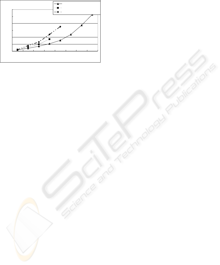
our approach divides the transaction into smaller

parts, it can solve the problem of long transactions.

100

150

200

250

300

5 10152025303540

The length of transaction

Runtime(sec)

Our approach

FSE

Item-Transformation A

roach

Figure 3: Runtime test for different length of transactions.

5 CONCLUSIONS AND FUTURE

WORK

Here are the advantages of our approach:

(1) Scan the database only once.

(2) No generation of candidates from

previously found frequent itemsets since

our approach directly enumerates all

candidates with efficient indexing for

support counting.

(3) No need to set support thresholds in

advance because we keep support counts

for all possible interesting itemsets.

(4) The result generated by our approach is

sorted by the support count such that

users can find what they want easily.

(5) No candidate itemset is generated if it

does not appear in the transactions.

(6) Our method has the same degree of

complexity as the FSE. However, the

processing cost is not proportional to the

length of the itemset.

(7) Our method is an incremental mining

approach. New items can be processed

in a regular manner.

We have implemented our algorithm and studied

its performance in comparison with other algorithms

for various sizes of databases. Our approach

outperforms the other algorithms.

In the future, we plan to improve the efficiency

of processing and retrieving the support counters of

the candidate itemsets with more direct access

approach. We will also apply our approach in the

parallel frequent pattern mining (Agrawal, 1996) and

sequential patterns mining (

Srikant, 1996; Pei, 2004).

ACKNOWLEDGEMENTS

This work was supported in part by the National

Science Council, Taiwan, under Grants NSC96-

2218-E-007-007 and NSC95-2221-E-035-068-MY3.

REFERENCES

Agrawal, R. & Srikant, R., 1994. Fast Algorithms for

Mining Association Rules. Proc. of the 20th Intl. Conf.

on Very Large Data Bases, 487-499.

Agrawal, R., & Shafer, J. C., 1996. Parallel mining of

association rules. IEEE Transactions on Knowledge

and Data Engineering, 8, 6, 962-969.

Chu, T. P., Wu, F., & Chiang, S. W., 2005. Mining

Frequent Pattern Using Item-Transformation Method.

Fourth Annual ACIS Intl. Conf. on Computer and

Information Science, 698-706.

Cristoforr, L., 2008. ARtool Project. URL:

http://www.cs.umb.edu/~laur/ARtool/.

Dunkel, B., & Soparkar, N., 1999. Data Organization and

Access for Efficient Data Mining. Proc. of the 15th

Intl. Conf. on Data Engineering. 522-529.

Han, J. W., Pei, J., & Yin, Y. W. 2000. Mining frequent

patterns without candidate generation. SIGMOD

Record, 29, 1-12.

Hipp, J., Güntzer, U., Nakhaeizadeh, G., 2000. Algorithms

for Association Rule Mining - A General Survey and

Comparison. SIGKDD Explorations, 2, 1, 58-64.

IBM Almaden Research Center, 2006. Synthetic Data

Generator.URL:http://www.almaden.ibm.com/softwar

e/quest/

Lin, H. W., Yang, D. L., Liao, W. C., & Wu, J., 2007.

Efficient Support Counting of Candidate Itemsets for

Association Rule Mining. Proc. of the 2nd Intl.

Workshop on Chance Discovery and Data Mining,

190-196.

Pei, J., Han, J. W., Mortazavi-Asl, B., Wang, J. Y., Pinto,

H., Chen, Q. M., Dayal, U., & Hsu, M. C., 2004.

Mining sequential patterns by pattern-growth: The

PrefixSpan approach. IEEE Transactions on

Knowledge and Data Engineering, 16, 1424-1440.

Srikant, R., & Agrawal, R., 1996. Mining Sequential

Patterns: Generalization and Performance

Improvements. In Proc. of EDBT’96, 3–17.

Wang, J. Y., Han, J. W., Lu, Y., & Tzvetkov, P., 2005.

TFP: An efficient algorithm for mining top-K frequent

closed itemsets. IEEE Transactions on Knowledge and

Data Engineering, 17, 652-664.

EFFICIENT SUPPORT COUNTING OF CANDIDATE ITEMSETS FOR ASSOCIATION RULE MINING

185