METRICS FOR A MODEL DRIVEN DEVELOPMENT CONTEXT
Motoshi Saeki
Tokyo Institute of Technology, Ookayama 2-12-1-W8-83, Meguro, Tokyo 152-8552, Japan
Haruhiko Kaiya
Shinshu University, Wakasato 4-17-1, Nagano 380-8553, Japan
Keywords:
Metrics, Model Transformation, Graph Rewriting, Model Driven Development.
Abstract:
In a Model Driven Development context, in addition to the metrics of models themselves, the metrics of
model transformation should be considered in order to measure its various characteristics such as quality. In
this paper, we propose the technique to define the metrics of model transformation using a meta-modeling
technique and a graph rewriting techniques. The meta-modeling technique is used for defining model-specific
metrics, while graph rewriting rules formalize transformation. The values of model-specific metrics to be
calculated are attached to graph rewriting rules, and can be evaluated and propagated between the models
during the transformation. The evaluation and propagation methods can be defined within the graph rewriting
rules, and their evaluation and propagation result in the metric values of the transformation. Furthermore the
paper includes the example of transforming object models into relational database models in order to show the
usefulness of our approach.
1 INTRODUCTION
The techniques of metrics are to quantify characteris-
tics of software products and development processes,
e.g. quality, complexity, stability, development ef-
forts, etc., and are significant to predict these charac-
teristics at earlier steps of the development processes,
as well as to know the current status of the products
and the processes.
Model Driven Development (MDD) is one of the
promising approaches to develop software of high
quality with less developers’ efforts. There are wide
varieties of models such as object-oriented models,
data flow models, activity models etc. that can be
produced in the MDD processes. For example, object
oriented modeling mainly adopts class diagrams con-
sisting of classes and their associations, while in data
flow modeling data flow diagrams having processes
(data transformation), data flows and data stores, etc.
are used. In this situation, according to models, we
should use different metrics to quantify their charac-
teristics, and it is necessary to define the metrics ac-
cording to the models. For example, in the object-
oriented models, we can use the CK metrics (Chi-
damber and Kemerer, 1994) to quantify the structural
complexity of a produced class diagram, while we use
another metrics such as Cyclomatic number (McCabe
and Butler, 1989) for an activity diagram of UML
(Unified Modeling Language). These examples show
that effective metrics vary on a model, and first of all,
we need a technique to define model-specific metrics
in MDD context.
In MDD, model transformation is one of the key
technologies (OMG, 2003; Kleppe et al., 2003; Mel-
lor and Balcer, 2003) for development processes, and
the techniques of quantifying the characteristics of
model transformation and its processes are neces-
sary to measure the development processes based on
MDD. Although we have several metrics for quanti-
fying traditional and conventional software develop-
ment processes such as staff-hours, function points,
defect density during software testing etc., they are
not sufficient to apply to model transformation pro-
cesses of MDD. In other words, we need the met-
rics specific to model transformation in addition to
model-specific metrics. Suppose that a metric value
can express the complexity of a model, like CK met-
rics, a change or difference between the metric values
13
Saeki M. and Kaiya H. (2008).
METRICS FOR A MODEL DRIVEN DEVELOPMENT CONTEXT.
In Proceedings of the Third International Conference on Evaluation of Novel Approaches to Software Engineering, pages 13-22
DOI: 10.5220/0001759000130022
Copyright
c
 SciTePress

before and after a model transformation can be con-
sidered as the improvement or declination of model
complexity. For example, the model transformation
where the resulting model becomes more complex is
not better and has lower quality from the viewpoint
of model complexity. This example suggests that we
can define a metric of a model transformation with a
degree of changing the values of model-specific met-
rics by it. Following this idea, the formal definition
of a transformation should include the definition of
model-specific metrics so that the metrics can be cal-
culated during the transformation.
Although we could find excellent techniques to
formalize model transformation of MDD until now,
there are quite few arguments on the significance of
clarifying and defining the metrics of model trans-
formation (Saeki and Kaiya, 2006). In (Merilinna,
2005), the relations between model transformation
and quality attributes was discussed. However, the
goal of this work is the usage of model transforma-
tion in order to generate a new model from the older
model when quality requirements were changed.
In this paper, we propose a technique to solve the
problem on how to define metrics of model transfor-
mation together with model-specific metrics. To real-
ize this technique, as mentioned before, we take the
following existing techniques;
1. Using a meta modeling technique to specify
model-specific metrics
Since a meta model defines the logical structure of
models, we specify the definition of metrics, in-
cluding its calculation technique, as a part of the
meta model. Thus we can define model-specific
metrics formally. We use Class Diagram plus Ob-
ject Constraint Language (OCL) to represent meta
models with metrics definitions.
2. Using a graph rewriting system to formalize
model transformation
Since we adopt Class Diagram to represent a meta
model, a model following the meta model is math-
ematically considered as a graph. Model trans-
formation rules can be defined as graph rewrit-
ing rules and the rewriting system can execute the
transformation automatically in some cases.
The metric values to be calculated are attached to
graph rewriting rules, and can be evaluated and prop-
agated between the models during the transforma-
tion. This evaluation and propagation mechanism is
similar to Attribute Grammar, and the evaluation and
propagation methods can be defined within the graph
rewriting rules. We define the metrics of a model
transformation using the model-specific metric values
of the models, which are attached to the rules.
The usages of the meta modeling technique for
defining model-specific metrics (Saeki, 2003) and of
graph rewriting for formalizing model transformation
(Czarnecki and Helsen, 2003; Karsai and Agrawal,
2003; Saeki, 2002) are not new. In fact, OMG is
currently developing a meta model that can spec-
ify software metrics (OMG, 2006) and the workshop
(B´ezivin et al., 2006) to evaluate practical usability
of model transformation techniques including graph
rewriting systems was held. However, but the contri-
bution of this paper is the integrated application tech-
nique of meta modeling and graph rewriting to solve
the new problem, i.e. how to formalize the metrics of
model transformation, with unified framework.
The rest of the paper is organized as follows. In
the next section, we introduce our meta modeling
technique so as to define model-specific metrics. In
section 3, we briefly introduce graph rewriting tech-
nique to formalize model transformation. Section 4
presents the technique to define the metrics of model
transformation and includes the examples of the met-
rics of model transformations. Section 5 is a conclud-
ing remark and discusses the future research agenda.
2 META MODELING AND
DEFINING METRICS
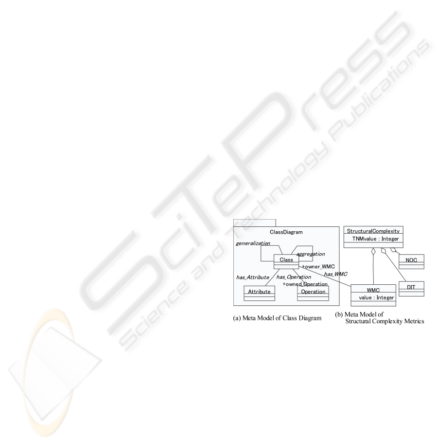
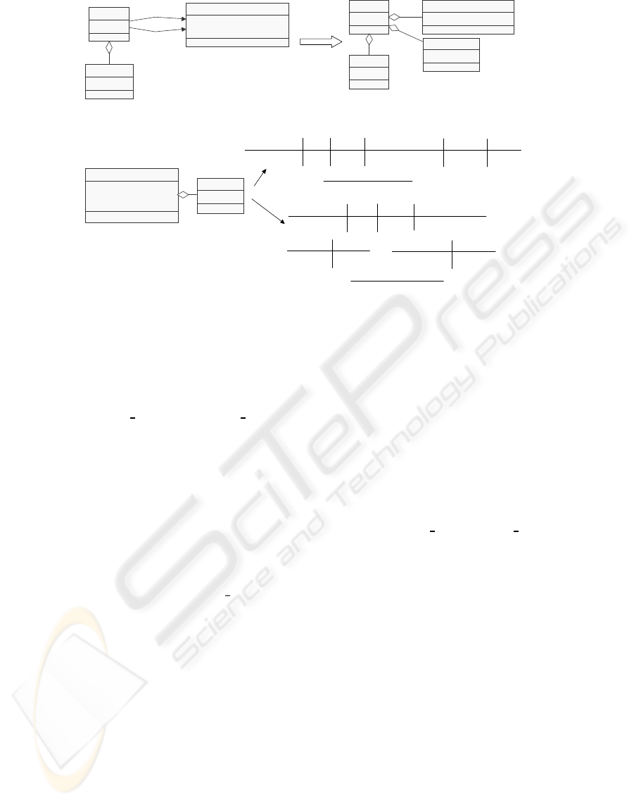
Figure 1: Meta Model with Metrics Definitions.
A meta model specifies the structure or data type of
the models and in this sense, it can be considered as
an abstract syntax of the models. In addition to meta
models, we should consider constraints on the mod-
els. Suppose that we define the meta model of the
models which are described with class diagrams, i.e.
object-oriented models. In any class diagram, we can-
not have different classes having the same name, and
we should specify this constraint to keep consistency
of the models on their meta model.
In our technique, we adopt a class diagram of
UML for specifying meta models and OCL for con-
straints on models. The example of the meta model
ENASE 2008 - International Conference on Evaluation of Novel Approaches to Software Engineering
14

of the simplified version of class diagrams is shown
in Figure 1 (a). As shown in the figure, it has the con-
cepts “Class”, “Operation” and “Attribute” and all of
them are defined as classes and these concepts have
associations representing logical relationships among
them. For instance, the concept “Class” has “At-
tribute”, so the association “has Attribute” between
“Class” and “Attribute” denotes this relationship.
We can embed metrics and their calculation meth-
ods into a meta model in the same way. More con-
cretely, metrics such as WMC (Weighted Methods per
Class), DIT (Depth of an Inheritance Tree) and NOC
(Number of Children) of CK metrics are defined as
classes having the attribute “value” in the meta model
as shown in the Figure 1 (b). The “value” has the met-
ric value and its calculation is defined as a constraint
written with OCL. For example, WMC is associated
with each class of a class diagram through the associ-
ation “has WMC” and the role names “owner WMC”
and “owned Operation” are employed to define the
value of WMC with OCL. Intuitively speaking, the
value of WMC is the number of the methods in a class
when we make weighted factors 1 and we take this
simple case. It can be defined as follows.
context WMC::value : Integer
derive: owner WMC.owned Operation -> size()
WMC and the other CK metrics are for a class not
for a class diagram. Thus we can use the maximum
number of WMCs in the class diagram or the average
value to represent the WMC for the whole of the class
diagram. In this example, which is used throughout
the paper, we take the sum total of WMCs for the class
diagram, and the attribute TNMvalue of Structural-
Complexity holds it as shown in Figure 1 (b). The
techniques of using OCL on a meta model to specify
metrics were also discussed in (Abreu, 2001; Saeki,
2003), and the various metrics for UML class dia-
grams can be found in (Genero et al., 2005).
3 GRAPH REWRITING SYSTEM
In Model Driven Development, one of the techni-
cally essential points is model transformation. Since
we use a class diagram to represent a meta model,
a model, i.e. an instance of the meta model can be
considered as a graph, whose nodes have types and
attributes, and whose edges have types, so called at-
tributed typed graph. Thus in this paper, model trans-
formation is defined as a graph rewriting system, and
graph rewriting rules dominate allowable transforma-
tions. In this section, we introduce a graph rewriting
system.
A graph rewriting system converts a graph into an-
other graph or a set of graphs following pre-defined
rewriting rules. There are several graph rewriting sys-
tems such as PROGRESS (Schurr, 1997) and AGG
(Taentzer et al., 2001). Since we should deal with
the attribute values attached to nodes in a graph, we
adopt the definition of the AGG system in this paper.
A graph consists of nodes and edges, and type names
can be associated with them. Nodes can have attribute
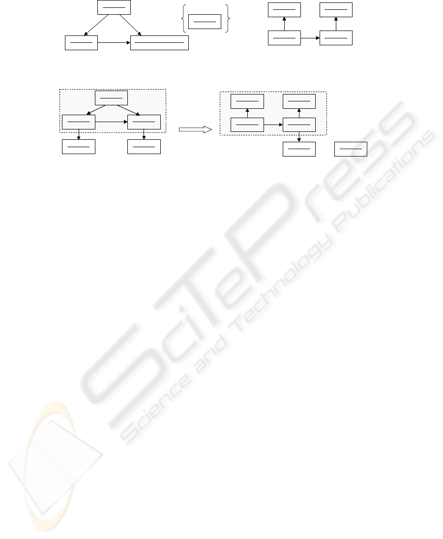
values depending on their type. The upper part of Fig-
ure 2 is a simple example of rewriting rules. A rule
consists of a left-hand and a right-hand side which
are separated with “::=”. The attribute values should
be able to be propagated in any direction, i.e. from
the left-hand side of “::=” to the right-hand side, the
opposite direction, as well as within the same side,
and this mechanism is similar to synthesized and in-
herited attributes of Attribute Grammar. In this sense,
the graph rewriting system that we use is an extended
version of AGG.
In figure 2, a rectangle box stands for a node of a
graph and it is separated into two parts with a hori-
zontal bar. Type name of a node appears in the upper
part of the horizontal bar, while the lower part con-
tains its attribute values. In the figure, the node of
“TypeA” in the left-hand graph has the attribute “val”
and its value is represented with the variable “x”. A
graph labeled with NAC (Negative Application Con-
dition) appearing in the left-hand controls the appli-
cation of the rule. If a graph includes the NAC graph,
the rule cannot be applied to it. In addition, we add
the conditions that are to be satisfied when the rule is
applied. In this example, we have two conditions, one
of which says that “val” of the node “1:TypeA” has to
be greater than 4 to apply this rewriting rule.
The lower part of Figure 2 illustrates graph rewrit-
ing. The part encircled with a dotted rectangular box
in the left-hand is replaced with the sub graph that is
derived from the right-hand of the rule. The attribute
values 5 and 2 are assigned to x and y respectively,
and those of the two instance nodes of “TypeD” re-
sult in 7 (x+y) and 3 (x-y). The attribute “val” of
“TypeD” node looks like an inherited attribute of At-
tribute Grammar because its value is calculated from
the attribute values of the left-hand side of the rule,
while “sval” of “TypeC” can be considered as a syn-
thesized attribute. The value of “sval” of the node
“TypeC” in the left-hand side is calculated from the
values in the right-hand side, and we get 8 (TypeD val
+ x = 3+5). Note that the value of “val” of “TypeA”
is 5, greater than 4, the value of “sval” is less than 10,
and none of nodes typed with “TypeD” appear, so the
rule is applicable. The other parts of the left-hand side
graph are not changed in this rewriting process.
METRICS FOR A MODEL DRIVEN DEVELOPMENT CONTEXT
15

TypeA
val =5
TypeB
val = 2
TypeC
a
b
b
TypeA
val =5
TypeB
val = 2
TypeC
a
b
b
TypeA
TypeB
TypeD TypeD
val=5 val=2
val=7 val=3
a
a
c
TypeE TypeA
c a
TypeE
TypeA
c
1:TypeA
val =x
2:TypeB
val = y
TypeC
a
b
b
1:TypeA
2:TypeB
TypeD TypeD
val=x val=y
val=x+y val=x-y
a a
c
1:TypeA
2:TypeB
TypeD TypeD
val=x val=y
val=x+y val=x-y
a a
c
:: =
TypeD
NAC
Rewriting Rule
Rewriting
1:TypeA_val > 4
TypeC_sval < 10
sval = TypeD_val + x
sval = 8
Figure 2: Graph Rewriting Rules and Rewriting Process.
4 METRICS ON MODEL
TRANSFORMATION
4.1 Using Model-Specific Metrics
The model following its meta model is represented
with an attributed typed graph and it can be trans-
formed by applying the rewriting rules. We call this
graph instance graph in the sense that the graph is an
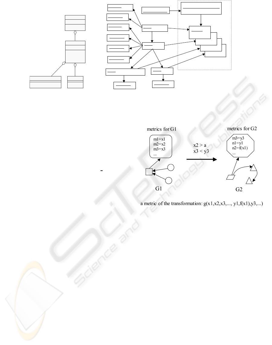
instance of the meta model. Figure 3 shows the ex-
ample of a class diagram of Lift Control System and
its instance graph following the meta model of Figure
1. The types of nodes result from the elements of the
meta model such as Class, Attribute and Operation,
while the names of classes, attributes and operations
are specified as the values of the attribute “name”. In
the figure, the class Lift in the class diagram corre-
sponds to the node typed with Class and whose at-
tribute “name” is Lift. Some nodes in the instance
graph have metric values as their attribute values. For
example, a node typed with WMC has the attribute
“value” and its value is the number of the operations
of the class, which is automatically calculated using
the formula (1). The WMC value of class Lift is 3 as
shown in the figure.
We can design graph rewriting rules considering
the nodes of the metrics and their values. See an
example of a transformation rule shown in Figure 4.
Two conditions x2 > a and x3 < y3 are attached to the
rule for rewriting the graph G1 with G2 and these con-
ditions should be satisfied before the rule is applied.
This transformation rule includes two nodes named
“metrics for G1” and “metrics for G2”, each of which
holds the metric values of the model. The first condi-
tion x2 > a expresses that the rule cannot be applied
until the value of the metric m2 before the rewriting is
greater than a certain value, i.e. “a”. It means that this
model transformation is possible when the model has
a metric value higher than a certain standard. The sec-
ond condition x3 < y3 specifies monotonic increasing
of the metric m3 in this transformation. This formula
has both metric values before and after the transfor-
mation as parameters and it can specify the charac-
teristics of the transformation, e.g. a specific metric
value is increasing by the transformation. As shown
in the figure, the calculation of the metric n2 uses the
metric m1 of the model before the transformation, and
this calculation formula of n2 shows that the metric
value of G1 is propagated to G2. The metrics of a
transformation can be formally specified by using this
approach. In Figure 4, we can calculate how much a
metric value could be improved with the transforma-
tion by using the metric values of the model before
the transformation and those after the transformation.
The function g in the figure calculates the improve-
ment degree of the metric value. This is a basic idea
of the metrics of model transformation.
Let’s consider the example of a model transfor-
mation using graph rewriting rules. The model of Lift
Control System in Figure 3 (a) can be considered as
a platform independent model (PIM) because of no
consideration of implementation situation, and we il-
lustrate its transformation into a platform dependent
model (PSM). We have a scheduler to decide which
lift should be made to come to the passengers by the
information of the current status of the lifts (the po-
sition and the moving direction of the lift), but we
don’t explicitly specify the concrete technique to im-
ENASE 2008 - International Conference on Evaluation of Novel Approaches to Software Engineering
16

:WMC
value = 1
:WMC
value = 1
:WMC
value = 1
:WMC
value = 1
:Class
name=Scheduler
:Class
name=EmergencyButton
:Operation
name=push
:Operation
name=arrived
:Class
name=Door
:Operation
name=request
:Operation
name=down
:Operation
name=up
:Attribute
name=position
:Class
name=Lift
:StructuralComplexity
:ClassDiagram:ClassDiagram
:Operation
name=open
:WMC
value = 3
:WMC
value = 3
:WMC
value = 1
:WMC
value = 1
(a) Class Diagram
(b) Instance Graph with Metrics Nodes
TNMvalue = 6
Door
open()
Scheduler
lift_status
arrived()
Lift
position
up()
down()
request()
EmergencyButton
push()
:Attribute
name=lift_status
Metrics NodesMetrics Nodes
Figure 3: Class Diagram and Its Instance Graph.
plement the function of getting the status information
from the lifts. If the platform that we will use has
an interrupt-handling mechanism to detect the arrival
of a lift at a floor, we put a new operation “notify”
to catch the interruption signal in the Lift module.
The notify operation calls the operation “arrived” of
Scheduler and the “arrived” updates the lift status at-
tribute according to the data carried by the interrupt
signal. As a result, we can get a PSM that can oper-
ate under the platform having interrupt-handlingfunc-
tions. In Figure 5, Rule #1 is for this transformation
and PSM#1 is the result of applying this rule to the
PIM of Lift Control System.
Another alternative is for the platform without
any interrupt-handling mechanism, and in this plat-
form, we use multiple instances of a polling routine
to get the current lift status from each lift. The class
Thread is an implementation of the polling routine
and its instances are concurrently executed so as to
monitor the status of the assigned lift. To execute a
thread object, we add the operations “start” for start-
ing the execution of the thread and “run” for defin-
ing the body of the thread. The operation “attach”
in Scheduler is for combining a scheduler object to
the thread objects. Rule #2 and PSM#2 in the fig-
ure specifies this transformation and its result respec-
tively. The TNMvalue, the total sum of the opera-
tions, can be calculated following the definition of
Figure 1 for PIM, PSM#1 and PSM#2. It can be con-
sidered that the TNM value expresses the efforts to
implement the PSM because it reflects the volume of
the source codes to be implemented. Thus the differ-
ence of the TNMvalues (∆TNMvalue) between the
PIM to the PSM represents the increase of implemen-
tation efforts. In this example, PSM#1 is easier to
implement because ∆TNMvalue of PSM#1 is smaller
than that of PSM#2, as shown in Figure 5. So we
Figure 4: Metrics and Model Transformation.
can conclude that the transformation Rule #1 is bet-
ter rather than Rule #2, only from the viewpoint of
less implementation efforts. This example suggests
that our framework can specify formally the metrics
of model transformations by using the metric values
before and after the transformations.
4.2 Example: Transforming a Class
Model to Relational Tables
In the previoussection, we showed the example where
the model metrics before and after the transforma-
tion were used to calculate the metrics of the trans-
formation. On the other hand, in this section, we
pick up more complicated example of metrics of
transformation that are defined using the values of
the model metrics before or during the transforma-
tion. Our example is based on the mandatory exam-
ple of Workshop on Model Transformations in Prac-
tice jointly held in MoDELS/UML2005 Conference
(B´ezivin et al., 2006) and it is the transformation of
METRICS FOR A MODEL DRIVEN DEVELOPMENT CONTEXT
17

:StructuralComplexity
:ClassDiagram:ClassDiagram
TNMvalue = m
:Class
name=x
:Class
name=x
:Class
name=y
:Class
name=y
:Class
name=Thread
:Class
name=Thread
:Operation
name=notify
:Operation
name=notify
:Operation
name=attach
:Operation
name=attach
:Operation
name=start
:Operation
name=start
:Operation
name=run
:Operation
name=run
:Class
name=x
:Class
name=x
:Class
name=y
:Class
name=y
:Class
name=x
:Class
name=x
:Class
name=y
:Class
name=y
:Class
name=x
:Class
name=x
:Class
name=y
:Class
name=y
monitors
:StructuralComplexity
:ClassDiagram:ClassDiagram
TNMvalue = n
:StructuralComplexity
:ClassDiagram:ClassDiagram
TNMvalue = n
:StructuralComplexity
:ClassDiagram:ClassDiagram
TNMvalue = m
Scheduler
lift_status
arrived()
Lift
notify()
Scheduler
lift_status
arrived()
attach()
Lift
Thread
start()
run()
monitors
Lift
Scheduler
lift_status
arrived()
::=
::=
Rule#1
Rule#2
Transformation from a PIM to a PSM
ΔTNMvalue = n-m = 1
ΔTNMvalue = n-m = 3
PIM
PSM#1
PSM#2
Rule#1
Rule#2
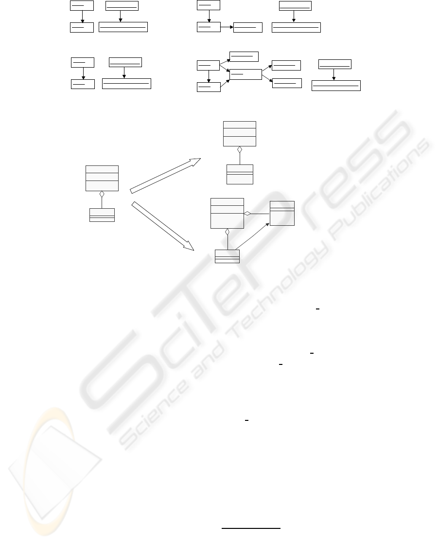
Figure 5: Model Transformation Example.
a class model into a relational database. More con-
cretely, a set of tables for a relational database, i.e.
schema is generated from a class model. Figure 6
shows the overview of this example. The meta mod-
els of class diagrams and of relational tables (shortly
tables) are shown in the figure (a). An association in
the meta model of class diagrams has cardinalities as
its attributes and the value of cardinality consists of a
pair of integers; minimal and maximal cardinalities.
As shown in the meta model of tables, a table con-
sists of one or more columns. Note that two elements
StructuralComplexity and Redundancy are associated
to Table and will be used for the calculation of met-
rics.
We can have two alternatives of transformation as
shown in Figure 6 (b). The first alternative is sim-
pler and it produces a single and flat table from a
class diagram, while a set of tables with less redun-
dant data entries is generated in the second alterna-
tive. Let us explain the example of Customer-Order
class diagram shown in the left-hand side of Figure
6 (b). In the first alternative of transformation, we
generate a table where all of the classes and their at-
tributes are included and formed in a line of columns.
More concretely,all of object identifiers and attributes
are collected into a single table. For Customer class,
the identifier Customer ID, “name”, “address” and
“telephone-number” are extracted and put as columns
of a table. As for Order class, the transformation adds
its identifier and attributes. The resulting table has
the columns Customer ID, name, address, telephone-
number, Order ID and amount, as shown in the figure
(b) (1). It may have redundant data entries. For exam-
ple, suppose that a customer has more than one order,
say 100 orders. The table has the 100 entries but they
include the 100 occurrences of the same data of Cus-
tomer ID, name, address and telephone-number. This
type of the table is so called first normal form. On the
other hand, the second alternative is the transforma-
tion for reducing redundant data entries. As shown in
Figure 6 (b) (2), for each class and association, a ta-
ble is generated. In this example, we have three tables
Customer, Order and Customer-Order, and they are in
third normal form
1
.
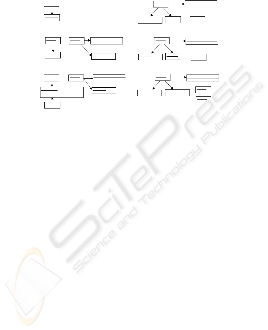
A part of the rules for these two transformations is
shown in Figures 7 and 8 respectively. For simplicity,
1
If the attributes that are not so dependent on a class
exist, the tables may not be in third normal form but sec-
ond one. For example, if Customer class has the attribute
“mayor’s name in the home address” in addition to “(home)
address”, its transformation result is in second normal form,
because a mayor essentially depends not on a customer but
on his address.
ENASE 2008 - International Conference on Evaluation of Novel Approaches to Software Engineering
18

Customer_ID name address telephone-number
Order_ID amountOrder_ID amount
Customer_ID Order_IDCustomer_ID Order_ID
(a) Meta Model
(b) Transformation from a Class Diagram to Tables
(1) First Normal Form
(2) Third Normal Form
Class Diagram
Relational Table (Schema)
Attribute
name
Association
source _cardinality
destination_cardinality
Class
name
source
destination
name
Order
amount
Customer
name
address
telephone-number
Customer_ID name address telephone-number Order_ID amountCustomer_ID name address telephone-number Order_ID amount
Column
name
StructuralComplexity
val
Redundancy
val
Table
name
Figure 6: A Class Model and Relational Tables.
we omit NAC parts from the rules. The rules in Fig-
ure 7 is for performing the transformation shown in
Figure 6 (b) (1). By Rule #1, a table having an object
identifier (class name + ID, e.g. Customer ID) and
an attribute y as columns is initially created. Rule #2
is iteratively applied according to the occurrences of
the attributes in the class x and this rule adds them to
a table as its columns. This iterative application con-
tinues until all attributes of class x have been added
to the table. To deal with the occurrences of associ-
ations between classes, Rule #3 is iteratively applied
so that the object identifiers of the other classes, e.g.
y, are newly added to the table. The attributes of the
newly added class are also added in the same way us-
ing Rule #2. Note that i and j of a source cardinality
express the range of the cardinality, i.e. minimal and
maximal cardinalities of the class that is the source of
the association. In this transformation, we adopt the
metrics expressing the structural complexity of the ta-
ble and it is the sum of the number of the columns
plus 1. “Plus 1” means that we include the number
of the tables in the structural complexity. The calcu-
lation is being performed during the transformation,
and its result is in the attribute “val” of the node Struc-
turalComplexity, which is connected to the generated
table.
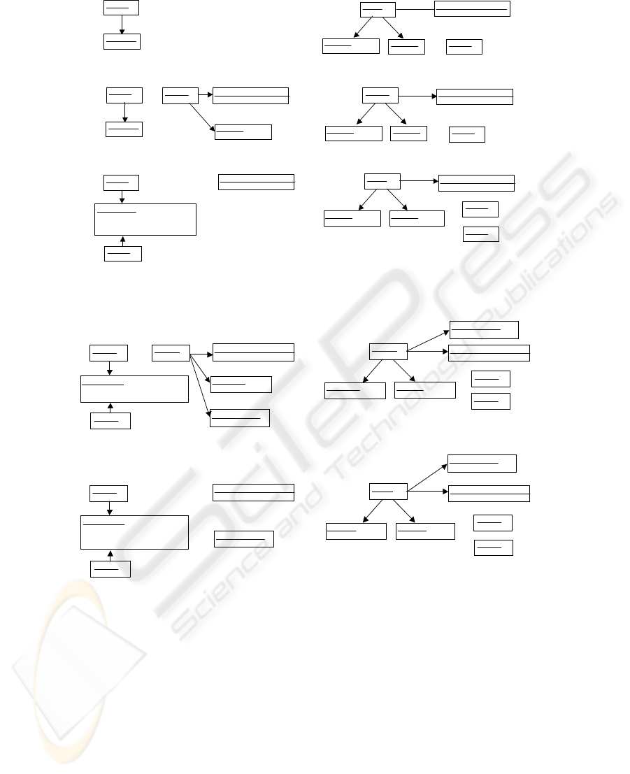
The rules shown in Figure 8 are for performing the
transformation in Figure 6 (b) (2) and for getting ta-
bles in third normal form. Rules #1 and #2 are quite
similar to the rules of the previous example, except
that the Table nodes have their names as represented
with “name=x” in the figure. These two rules gen-
erate a table for each class, and the generated table
includes as columns all attributes of the class. For ex-
ample, their applications generate Customer and Or-
der tables. To generate a table for each association
between two classes, e.g. x and y, Rule #3 is ap-
plied. The generated table consists of two columns,
each of which is an object identifier of the class par-
ticipating in the association. For example, from an
association between Customer and Order, as shown
in Figure 6 (2) (b), we can get a table having the two
columns Customer ID and Order ID. To quantify a
characteristic of transformation, we pick up structural
complexity of the resulting tables, which is calculated
with a total number of the tables and columns.
From structural complexity view, the transforma-
tion (1) generating a table of first normal form is bet-
ter than (2), because it generates only one table and
fewer columns. However, the table of first normal
form may have redundant data entries as mentioned
before. Lower cardinality the associations have, the
fewer redundant data entries can be included in the ta-
ble. For example, all associations appearing in a class
model have the cardinality 1, i.e. they are one-to-one
associations, the table of first normal form, which has
been generated by Figure 7, cannot have any redun-
dant data entries. So, it is better that we add to our
metrics the degree of the possibility of including re-
dundant data entries in the resulting tables. To com-
plete our metrics, using the maximal cardinality val-
ues j and k in Figures 7 and 8, we calculate how many
redundant data entries can appear in the tables. Fig-
ure 9 shows the transformation rules to calculate the
METRICS FOR A MODEL DRIVEN DEVELOPMENT CONTEXT
19

1:Class
name=x
1:Class
name=x
:Attribute
name=y
:Attribute
name=y
:Table:Table
:StructuralComplexity
val = 1+1
:StructuralComplexity
val = 1+1
::=
1:Class
name=x
1:Class
name=x
2:Class
name=y
2:Class
name=y
::=
:Column
name=y
:Column
name=y
3:Table3:Table
:Association
source_cardinality = (i,j)
destination_cardinality = (l.k)
:Association
source_cardinality = (i,j)
destination_cardinality = (l.k)
1:Class
name=x
1:Class
name=x
5:StructuralComplexity
val = n+1
5:StructuralComplexity
val = n+1
1:Class
name=x
1:Class
name=x
3:Table3:Table
2:Class
name=y
2:Class
name=y
5:StructuralComplexity
val = n
5:StructuralComplexity
val = n
Rule#1
Rule#3
1:Class
name=x
1:Class
name=x
:Attribute
name=y
:Attribute
name=y
:StructuralComplexity
val = n+1
:StructuralComplexity
val = n+1
::=
1:Class
name=x
1:Class
name=x
2:Table2:Table
3:StructuralComplexity
val = n
3:StructuralComplexity
val = n
Rule#2
2:Table2:Table
:Column
name=y
:Column
name=y
4:Column
name= x+”_ID”
4:Column
name= x+”_ID”
4:Column
name= x+”_ID”
4:Column
name= x+”_ID”
Column
name= x+”_ID”
Column
name= x+”_ID”
4:Column
name= x+”_ID”
4:Column
name= x+”_ID”
4:Column
name= x+”_ID”
4:Column
name= x+”_ID”
Column
name= y+”_ID”
Column
name= y+”_ID”
source
destination
Figure 7: Rules for Transformation (1): to First Normal Form.
metric of Redundancy, and we can use as a metric
of these transformations the weighted linear combi-
nation of StructuralComplexity and Redundancy. To
calculate it, we add the node having the value of the
Redundancymetric to the Rule #3 in both of the trans-
formations (1) and (2). In the transformation (1), the
number of redundant data entries depends on the max-
imal cardinalities of an association, and so we use the
multiplication of the cardinalities of source and des-
tination classes in the association. If the both cardi-
nalities are 1, there are no possibilities of occurring
redundant data entries, i.e. the redundancy value is 0.
The redundancy value of the resulting table is the total
sum of the redundancy values of all associations ap-
pearing in the class model. In the transformation (2),
the transformation of any association does not cause
this type of redundancy, and so our calculation does
not change the value of the node Redundancy, i.e. m,
as shown in Rule #3 for (2) in Figure 9.
This example uses not only the model metrics af-
ter the transformation, but also the model metrics be-
fore the transformation or of the intermediate artifacts
during the transformation. Note that we used two spe-
cific metrics StructuralComplexity and Redundancy
for the explanation of our technique. Readers can
find more useful and practical metrics for relational
databases, e.g. the number of foreign keys and the
depth of a referential tree in (Calero et al., 2001), and
our approach can be applied to them.
5 CONCLUSIONS AND FUTURE
WORK
In this paper, we propose the technique to specify
the metrics of model transformations based on graph
rewriting systems, and show the applicability of our
technique using the examples of model transforma-
tion. Our final goal of this research project is to
develop the techniques of measuring the quality of
model transformations in addition to of models. Al-
though the metrics that we picked up in this paper
were for quantifying complexity and could not ex-
press the quality directly, they surely affect the qual-
ity. Exploiting the metrics related to quality in a MDD
context is the next step of this project.
In addition, the future research agenda can be
listed up as follows.
1) Metrics on Graph Rewriting. The metrics men-
tioned in the previous section was based on model-
specific metrics and value changes during model
transformations. We can consider another type of
metrics based on characteristics of graph rewriting
rules. For example, the fewer graph rewriting rules
that implement the model transformation may lead the
more understandable transformation, and the com-
plexity of the rules can be used as the measure of
understandability of the transformation. This kind of
complexity such as the number of rules and the num-
ber of nodes and edges included in the rules can be
calculated directly from the rules. Another example
is related to the process of executing graph rewriting.
During a transformation process, we can calculate the
number of the application of rules to get a final model,
ENASE 2008 - International Conference on Evaluation of Novel Approaches to Software Engineering
20

1:Class
name=x
1:Class
name=x
:Attribute
name=y
:Attribute
name=y
:Table
name =x
:Table
name =x
:Column
name= x+”_ID”
:Column
name= x+”_ID”
:StructuralComplexity
val = 1+1
:StructuralComplexity
val = 1+1
::=
1:Class
name=x
1:Class
name=x
2:Class
name=y
2:Class
name=y
::=
:Column
name=y
:Column
name=y
:Table
name=z
:Table
name=z
:Column
name= y+”_ID”
:Column
name= y+”_ID”
:Association
name = z
source_cardinality = (i,j)
destination_cardinality = (l.k)
1:Class
name=x
1:Class
name=x
3:StructuralComplexity
val = n+2+1
3:StructuralComplexity
val = n+2+1
1:Class
name=x
1:Class
name=x
1:Class
name=x
1:Class
name=x
:Attribute
name=y
:Attribute
name=y
3:StructuralComplexity
val = n+1
3:StructuralComplexity
val = n+1
::=
1:Class
name=x
1:Class
name=x
2:Table
name=x
2:Table
name=x
3:StructuralComplexity
val = n
3:StructuralComplexity
val = n
2:Class
name=y
2:Class
name=y
3:StructuralComplexity
val = n
3:StructuralComplexity
val = n
Rule#1
Rule#2
Rule#3
2:Table
name=x
2:Table
name=x
:Column
name=y
:Column
name=y
:Column
name= x+”_ID”
:Column
name= x+”_ID”
:Column
name= x+”_ID”
:Column
name= x+”_ID”
:Column
name= x+”_ID”
:Column
name= x+”_ID”
source
destination
Figure 8: Rules for Transformation (2): to Third Normal Form.
1:Class
name=x
1:Class
name=x
2:Class
name=y
2:Class
name=y
::=
:Table
name=z
:Table
name=z
:Column
name= y+”_ID”
:Column
name= y+”_ID”
:Association
name = z
source_cardinality = (i,j)
destination_cardinality = (l.k)
3:StructuralComplexity
val = n+2+1
3:StructuralComplexity
val = n+2+1
1:Class
name=x
1:Class
name=x
2:Class
name=y
2:Class
name=y
3:StructuralComplexity
val = n
3:StructuralComplexity
val = n
Rule#3 for (2)
:Column
name= x+”_ID”
:Column
name= x+”_ID”
1:Class
name=x
1:Class
name=x
2:Class
name=y
2:Class
name=y
::=
3:Table3:Table
:Association
source_cardinality = (i,j)
destination_cardinality = (l.k)
:Association
source_cardinality = (i,j)
destination_cardinality = (l.k)
5:StructuralComplexity
val = n+1
5:StructuralComplexity
val = n+1
1:Class
name=x
1:Class
name=x
3:Table3:Table
2:Class
name=y
2:Class
name=y
5:StructuralComplexity
val = n
5:StructuralComplexity
val = n
Rule#3 for (1)
4:Column
name= x+”_ID”
4:Column
name= x+”_ID”
4:Column
name= x+”_ID”
4:Column
name= x+”_ID”
Column
name= y+”_ID”
Column
name= y+”_ID”
6:Redundancy
val = m
6:Redundancy
val = m
4:Redundancy
val = m
4:Redundancy
val = m
6:Redundancy
val = m+((j*k)-1)
6:Redundancy
val = m+((j*k)-1)
4:Redundancy
val = m
4:Redundancy
val = m
source
source
destination
destination
Figure 9: Metric for Redundancy.
and this measure can express efficiency of the model
transformation. The smaller the number is the more
efficient. This type of metrics is apparently different
from the above metrics on the complexity of rules, in
the sense that it is the metrics related to the actual ex-
ecution processes of transformation. We call the for-
mer type of the metrics static metrics and the latter
dynamic one. As mentioned above, our approach has
potentials for defining wide varieties of model trans-
formation metrics.
2) Development of Supporting Tools. We consider
the extension of the existing AGG system, but to sup-
port the calculation of the metrics of transformations
and the selection of suitable transformations, we need
more powerful evaluation mechanisms of attribute
values. The mechanisms for version control of mod-
els and re-doing transformations are also necessary to
make the tool practical.
3) Usage of Standards. For simplicity, we used class
diagrams to represent meta models and OCL to de-
fine metrics. To increase the portability of meta mod-
els and metrics definitions, we will adapt our tech-
nique to standard techniques that OMG proposed or is
proposing, i.e. MOF, XMI, QVT and Software Met-
rics Metamodel (OMG, 2006).
4) Collecting Useful Definitions of Metrics. In the
METRICS FOR A MODEL DRIVEN DEVELOPMENT CONTEXT
21

paper, we illustrated very simple metrics for expla-
nation of our approach. Although the aim of this re-
search project is not to find and collect useful and ef-
fective metrics, making a kind of catalogue of metric
definitions and specifications like (Ebert et al., 2005;
Lorenz and Kidd, 1994) is important in the next step
of the supporting tool. The assessment of the col-
lected metrics is also a research agenda.
REFERENCES
Abreu, F. B. (2001). Using OCL to Formalize Object Ori-
ented Metrics Definitions. In Tutorial in 5th Interna-
tional ECOOP Workshop on Quantitative Approaches
in Object-Oriented Software Engineering (QAOOSE
2001).
B´ezivin, J., Rumpe, B., Schur, A., and Tratt, L. (2006).
Model Transformations in Practice Workshop. In Lec-
ture Notes in Computer Science, volume 3844, pages
120–127.
Calero, C., Piattini, M., and Genero, M. (2001). Empirical
Validation of Referential Integrity Metrics. Informa-
tion & Software Technology, 43(15):949–957.
Chidamber, S. and Kemerer, C. (1994). A Metrics Suite
for Object-Oriented Design. IEEE Trans. on Software
Engineering, 20(6):476–492.
Czarnecki, K. and Helsen, S. (2003). Classification of
Model Transformation Approaches. In OOPSLA2003
Workshop on Generative Techniques in the context of
Model Driven Architecture.
Ebert, C., Dumke, R., Bundschuh, M., and Schmietendorf,
A. (2005). Best Practices in Software Measurement.
Springer.
Genero, M., Piattini, M., and Calero, C. (2005). A Survey of
Metrics for UML Class Diagrams. Journal of Object
Technology, 4(9):59–92.
Karsai, G. and Agrawal, A. (2003). Graph Transformations
in OMG’s Model-Driven Architecture: (Invited Talk).
In AGTIVE, pages 243–259.
Kleppe, A., Warmer, J., and Bast, W. (2003). MDA Ex-
plained. Addison-Wesley.
Lorenz, M. and Kidd, J. (1994). Object-Oriented Software
Metrics. Prentice-Hall.
McCabe, T. and Butler, C. (1989). Design Complexity Mea-
surement and Testing. CACM, 32(12):1415–1425.
Mellor, S. and Balcer, M. (2003). Executable UML.
Addison-Wesley.
Merilinna, J. (2005). A Tool for Quality-
Driven Architecture Model Transformation.
http://virtual.vtt.fi/inf/pdf/publications/2005/P561.pdf.
OMG (2003). MDA Guide Version 1.0.1.
http://www.omg.org/mda/.
OMG (2006). ADM Software Metrics Metamodel RFP.
http://www.omg.org/docs/admtf/06-09-03.doc.
Saeki, M. (2002). Role of Model Transformation in Method
Engineering. In Lecture Notes in Computer Science
(Proc. of CAiSE’2002), volume 2348, pages 626–642.
Saeki, M. (2003). Embedding Metrics into Information
Systems Development Methods: An Application of
Method Engineering Technique. In Lecture Notes
in Computer Science (Proc. of CAiSE 2003), volume
2681, pages 374–389.
Saeki, M. and Kaiya, H. (2006). Model Metrics and Metrics
of Model Transformation: Materials of 1st Workshop
on Quality in Modeling: MoDELS2006 Conference.
http://www.ituniv.se/ miroslaw/QiM.htm.
Schurr, A. (1997). Developing Graphical (Software Engi-
neering) Tools with PROGRES. In Proc. of 19th Inter-
national Conference on Software Engineering (ICSE’
97), pages 618–619.
Taentzer, G., Runge, O., Melamed, B., Rudorf, M.,
Schultzke, T., and Gruner, S. (2001). AGG : The
Attributed Graph Grammar System. http://tfs.cs.tu-
berlin.de/agg/.
ENASE 2008 - International Conference on Evaluation of Novel Approaches to Software Engineering
22