Comparison of Adaboost and ADTboost
for Feature Subset Selection
Martin Drauschke and Wolfgang F
¨
orstner
Department of Photogrammetry, Institute of Geodesy and Geoinformation
University of Bonn, Nussallee 15, 53115 Bonn, Germany
Abstract. This paper addresses the problem of feature selection within classi-
fication processes. We present a comparison of a feature subset selection with
respect to two boosting methods, Adaboost and ADTboost. In our evaluation, we
have focused on three different criteria: the classification error and the efficiency
of the process depending on the number of most appropriate features and the
number of training samples. Therefore, we discuss both techniques and sketch
their functionality, where we restrict both boosting approaches to linear weak
classifiers. We propose a feature subset selection method, which we evaluate on
synthetic and on benchmark data sets.
1 Introduction
Feature selection is a challenging task during image interpretation, especially if the
images show highly structured objects with a rich diversity in variable environment,
where single variables are lowly correlated with the classification target. Also, feature
selection is used in data mining to extract useful and comprehensible information from
data, cf. [9]. One classical approach is principal component analysis, which reduces the
dimension of the feature space by projecting all features, cf. [1]. The resulting feature
set of a PCA is not a subset of all candidate features, but combinations of the original
features. Thus, the PCA is not an appropriate tool, if one wants to obtain a real subset
of features for further investigations. However, the feature weighting in Adaboost and
ADTboost may directly be used as a heuristic for feature selection. The paper inversti-
gates the potential of these two methods on synthetic and benchmark data.
Typically, one uses a data set of training samples to select a subset of appropriate
features and to train a classifier. Then, the effect of this feature selection and the clas-
sification is evaluated on a different data set, the test samples. There are three different
costs which have to be observed during this evaluation:
1. the classification error and
2. the efficiency of the process depending on
(a) the number of most appropriate features and
(b) the number of training samples.
Problem Specification. The problem can be formalized as follows: Given is a data
set of N training samples (x
n
, y
n
), where x
n
= [f
n
1
, .., f
n
D
] is a D-dimensional feature
Drauschke M. and Förstner W. (2008).
Comparison of Adaboost and ADTboost for Feature Subset Selection.
In Proceedings of the 8th International Workshop on Pattern Recognition in Information Systems, pages 113-122
Copyright
c
 SciTePress

vector of real numbers, and y
n
is the class membership. In this paper, we only con-
sidered the binary case, i. e. y
n
∈ {−1, +1}, but all applied algorithms have already
been introduced for the multi-class case, cf. [15] and [8], respectively. Our final goal
is not only the classification of these feature vectors, we additionally want to select the
best features to reduce the dimension of the feature space and to eliminate redundant
features.
Structure of the Paper. In section 2, we give a review on feature subset selection
principles and methods. Then, in section 3, we outline the Adaboost and ADTboost
algorithms and show their similarities and differences w. r. t. feature selection. Further-
more, we demonstrate and discuss their functionality regarding a simple example. Our
feature subset selection schemes with Adaboost and ADTboost are proposed in section
4. We have tested our approach on synthetic and benchmark data. The results of these
experiments are presented and discussed in section 5. Finally, we summarize our work
and give a short outlook of our research plans.
2 Standard Feature Selection Methods
If we want to select a subset of appropriate features from the total set of features with
cardinality D, we have a choice between 2
D
possibilities. If we deal with feature vectors
with more than a few dozens components, the exhaustive search takes too long. Thus,
we have to find other ways to select a subset of features.
One choice are genetic algorithms which select these subsets randomly. But al-
though they are relatively insensitive to noise, and there is no explicit domain knowl-
edge required, the creation of mutated samples within the evolutionary process might
lead to wrong solutions. Furthermore, the computational time of genetic algorithms in
combination with a wrapped classification method is not efficient, cf. [10].
Alternatively, there are deterministic approaches for selecting subsets of relevant
features. Forward selection methods start with an empty set and greedily add the best
of the remaining features to this set. Contrarily, backward elimination procedures start
with the full set containing all features, and then the most useless features are greedily
removed from this set. According to [11], feature subset selection methods can also get
characterized as filters and wrappers. Filters use evaluation methods for feature ranking
that are independent from the learning method. E. g. in [7], there the squared Pearson’s
Correlation Coefficient is proposed for determining the most relevant features.
In our experiments, the features have low correlation coefficients with the class
target and they are highly correlated with each other. Furthermore, the training samples
do not form compact clusters in feature space. Then, it is a hard task to find a single
classifier that is able to separate the two classes. Thus, we look for a wrapper method,
where the evaluation of the features is based on the learning results. Since we obtained
bad classification results using only one classifier, we would like to merge the feature
subset selection with a learning technique that uses several classifiers. This motivated
us to pursue the concept of adaptive boosting (Adaboost) where a strong (or highly
accurate) classifier is found by combining several weak (or less accurate) classifiers, cf.
[14].
114

Such majority voting is also used in random forests. The decision trees in [2] ran-
domly choose a feature from the whole feature set and takes it for determining the best
domain split. This method only works well, if the number of random decision trees
is large, especially if there are only features which are nearly uncorrelated with the
classes. In experiments of [2], there have been used five times more decision trees than
weak learners in Adaboost. Furthermore, if the number of decision trees is high, the
number of (randomly) selected features is also quite high. Then, we do not benefit on
feature subset selection, because almost every feature has been selected.
In [13], there is shown that ”the lack of implicit feature selection within random
forest can result in a loss of accuracy and efficiency, if irrelevant features are not re-
moved”. Therefore, we focus our work on Adaboost and ADTboost, which we briefly
summarize in the next chapter.
3 Adaboost and ADTboost
In this section, we recapitulate Adaboost and ADTboost in order to lay the basis for our
feature selection scheme. Furthermore, we demonstrate their functionality on a simple
example. For more details, we would like to refer to the original publications or our
technical report [4].
Adaboost. The concept of adaptive boosting (Adaboost) is to find a strong (or highly
accurate) classifier by combining several weak (or less accurate) classifiers, cf. [14].
The first weak classifier (or best hypothesis) is learnt on equally treated training sam-
ples (x
n
, y
n
). Then, before training the second weak classifier, the influence of all mis-
classified samples gets increased by adjusting the weights of the feature vectors. So, the
second classifier will focus especially on the previously misclassified samples. In the
third step, the weights are adjusted once more depending on the classification result of
the second weak classifier before training the third weak classifier, and so on.
Additionally, each weak classifier h
t
: x
n
7→ {+1, −1} is characterized by a pre-
dictive value α
t
which depends on the classifier’s success rate. After T weak classifiers
have been chosen, the result of the strong classifier H can be depicted as the sign of the
weighted sum of the results of the weak classifiers:
H(x
n
) = sign
X
t
α
t
h
t
(x
n
)
!
. (1)
The discriminative power of the resulting classifier H can be expected to be much
higher than the discriminative power of each weak classifier h
t
, cf. [12].
ADTboost. ADTboost is an extension of Adaboost which has been proposed in [6]
and refined in [3]. These extensions of Adaboost towards ADTboost are the following:
Primarily, the weak classifiers are put into a hierarchical order - the alternating decision
tree. The tree consists of two different kind of nodes which alternately change on a path
through the tree, cf. right part of fig. 1. Secondly, each decision node contains a weak
classifier and has two prediction nodes containing the predictive values α
+
t
and α
−
t
as its
115

children. The weak classifiers in upper levels of the tree work as preconditions on those
classifiers below them. And third, the root node contains the predictive value α
0
of the
true-classifier. Thus, α
0
is derived from the ratio of the number of samples between
both classes and, therefore, it can be interpreted as a a prior classifier. In each iteration
step, the best classifier candidate c
j
is determined in conjunction with a precondition
h
p
. Then, the new best weak classifier h
t
is set h
t
= h
p
∧c
j
. Furthermore, the prediction
of the t-th weak classifier is given by rule r
t
(x
n
), which is defined by
r
t
(x
n
) =



= α
+
t
, if h
p
(x
n
) = +1 and c
j
(x
n
) = +1
= α
−
t
, if h
p
(x
n
) = +1 and c
j
(x
n
) = −1
= 0, if h
p
(x
n
) = −1.
(2)
A Simple Example: Adaboost vs. ADTboost. We implemented Adaboost and ADT-
boost using the formulations of the algorithm in [15] and [3], respectively. Both al-
gorithms are optimized with respect to find the best weak classifier, to determine the
classifier’s weight or the predictive values, respectively, and to update each sample’s
weight. There are only two unsolved questions that are left to the user. The first question
refers to the maximum number of iterations. We stop the training either after T steps or
earlier, if the error rate on the training samples is below threshold θ. The other question
deals with the generation of the set of classifier candidates. Since we are interested in
the subset selection of the given features, we consider only threshold classification on
single features. Then, we avoid the combinatorial explosion which would occur, if we
would also consider linear seperation with 2 or more features.
Now, we want to discuss the functionality of both algorithms by presenting their
workflows on a synthetic data set, which is also visualized in fig. 1. It consists of points
which belong to two classes (red and blue). The target of the red class is y
n
= 1, and
the membership to blue class is encoded by y
n
= −1. We work with a 2-dimensional
feature vector, and its domain is x
n
∈ [0, 1] × [0, 1]. The class membership of a given
data point x
n
= [f
n
1
, f
n
2
] is defined by
y
n
=



+1 (red) - if f
n
1
< 0.4 and f
n
2
> 0.4 or
f
n
1
> 0.6 and f
n
2
< 0.6
−1 (blue) - else.
(3)
Besides the four domain bounds, we only need four other discriminative lines for
describing the feature set. Therefore, we limit our set of classifier candidates onto these
eight items: the domain bounds and
c
1
: if f
1
< 0.4 then red else blue
c
2
: if f
1
> 0.6 then red else blue
c
3
: if f
2
< 0.4 then red else blue
c
4
: if f
2
> 0.6 then red else blue
(4)
Since the calculations are documented in detail in [4], we only want to present
the results of Adaboost and ADTboost, respectively. Considering Adaboost, the final
predictions of the strong classifier after four iterations are obtained for a given x =
116

[f
1
, f
2
] by the sign of the weighted sums of the predicitions of all weak classifiers:
P
α
t
h
t
(x) f
1
< 0.4 0.4 ≤ f
1
≤ 0.6 f
1
> 0.6
f
2
> 0.6 −0.1149 −0.5203 0.1609
0.4 ≤ f
2
≤ 0.6 0.1849 −0.2205 0.4607
f
2
< 0.4 −0.1609 −0.5663 0.1149
. (5)
The bold entries in the table above document false predictions of the strong classi-
fier. This applies to 32% of the data. When proceeding with a larger set of candidates,
Adaboost could choose several other axis-parallel classifiers as f
1
< 0.5, and so the
classification could furtherly get improved.
The boosting process using alternating decision trees starts with a prior classi-
fication using the first predictive value α
0
= −0.04. Then, the we determine the
weak classifiers (including their precondition) in the following order: h
1
= true ∧c
1
,
h
2
= h
1
∧ ¬c
3
, h
3
= ¬h
1
∧ ¬c
4
and h
4
= h
3
∧ c
2
. After four iterations, the resulting
classifier has the in this example expected classification rate of 100%. And the strong
classifier determines the following predictions:
P
r
t
(x) f
1
< 0.4 0.4 ≤ f
1
≤ 0.6 f
1
> 0.6
0.6 ≤ f
2
0.79 −1.11 −0.57
0.4 < f
2
< 0.6 0.81 −1.09 1.62
f
2
≤ 0.4 −2.22 −1.09 1.62
. (6)
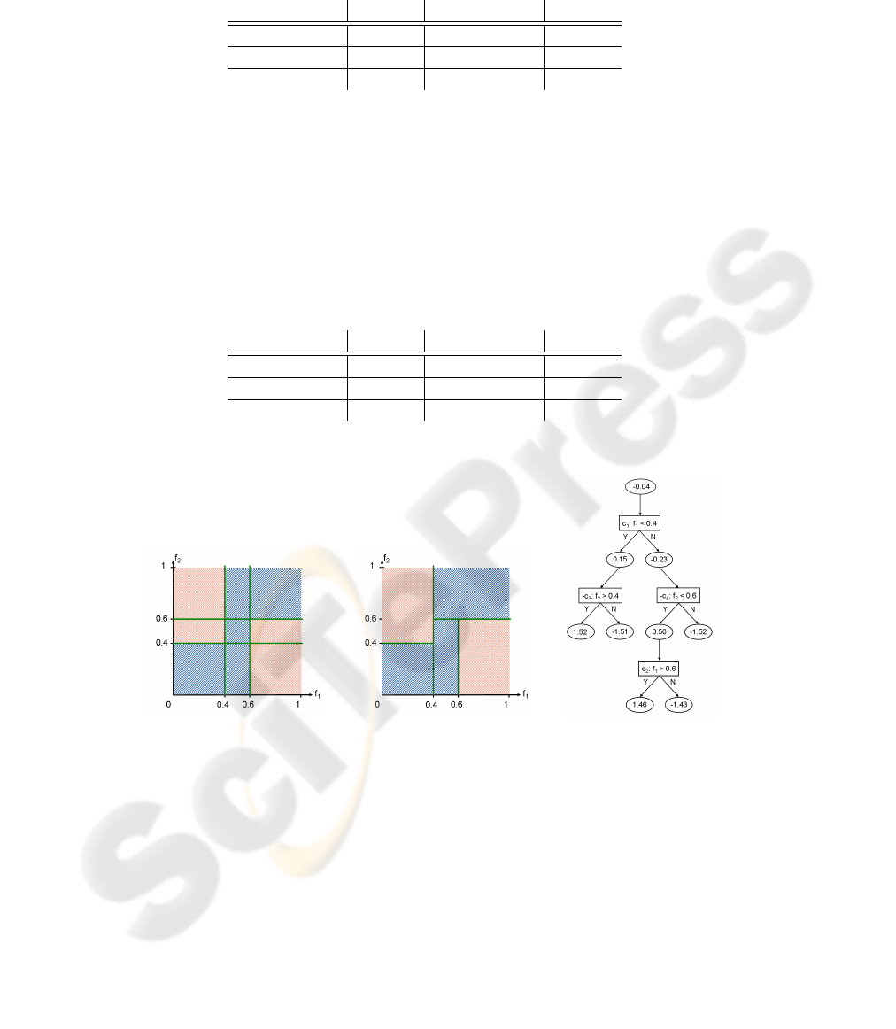
Fig. 1. Simple example with with 2 features and 2 classes (red and blue). Left: weak classifiers of
Adaboost. Middle: weak classifiers of ADTboost. Right: Alternating Decision Tree of ADTboost
result.
Comparison. Although we have demonstrated the functionality of Adaboost and
ADTboost on a very simple synthetic data set of two non-overlapping classes, we are
able to assert one major difference between both approaches. We designed our weak
classifiers such that each classification within Adaboost is a interpretable as a division
of the 2D feature space into two half spaces. The T linear classifiers form a partition
117

of the feature space into up to 2
T
sub-domains. The classification of all samples within
one sub-domain is equal, and the weak classifiers with the highest predictive values are
the most dominant one concerning the final result.
Alternatively, the hierarchical order of these weak classifiers builds a multiple k-d-
tree, see middle part of fig. 1. Multiple, because we could have several weak classifiers
with the same preconditions. In logical terms, the hierarchical compositions of classi-
fiers describe AND relations. If several classifiers have the same precondition, they are
composed by a OR relation.
ADTboost seems to favor to expand the alternating decision tree in depth. If the
classes do not overlap much, but form clusters of complex shapes, ADTboost will se-
lect fewer weak classifiers than Adaboost, if both methods are not terminated after a
predifined number of iterations, but when the error bounds fall below a certain thresh-
old. Unfortunately, this behavior of ADTboost also leads to overfitting. For avoiding
such overfitting, one could either restrict the depth of the alternating decision tree, or
the splitting must be done with respect to significant large subsets. So far, we have not
implemented such restrictions.
4 Feature Selection with Adaboost and ADTboost
If the number of iterations T is significantly less than the number of features D, then
the selection of the feature subset would be completed after the last iteration step. Then
we would have T weak classiers h
t
, and each of them performs a decision on a single
feature f
d(t)
. Hence, the set of these maximal T features is the relevant subset.
If the classification results only satisfy after many iterations with T ≈ D, then
(almost) all features could have been selected, and we do not necessarily obtain a subset
of the most relevant features so easily. In our point of view, we have two ways to derive
these most appropriate features.
In the first variant, we would search for the best weak classifiers until the maximal
cardinality of the feature subset is reached. In the further iterations, we restrict the
domain of the classifier candidates on these selected features. This strategy will lead to
a intervention of the classification process of Adaboost and ADTboost, and the feature
subset selection only depends on the time of choice of a weak classifier or a feature,
respectively, and not on their relevance or their effect on the strong classifier.
The second variant performs the feature subset selection after the learning has
stopped. Now, we evaluate the weak classifiers and their associated features after the
training of the strong classifier has finished. This will lead to the ranking of weak clas-
sifiers and their features, respectively. Considering Adaboost, the impact of each weak
classifier h
t
depends on the absolute value of α
t
. Then, the impact of a feature on the
classification result can be measured by its contributive value C which we define by
C (f
d
) =
X
t
|α
t
| where h
t
works on f
d
. (7)
When the subset of relevant features shall have a cardinality of S, S ≤ D, we choose
the S features with the highest contributive values. Regarding the simple example of
118

the previous section, we obtain C (f
1
) = 0.5433 and C (f
2
) = 0.3228. Thus, the best
feature is the first one.
When adapting this proposal, we need to integrate two predictive values for each
weak classifier, and we also need to consider the hierarchical order of the weak classi-
fiers. Thus, we re-define the contributive values by
C (f
d
) =
X
t
ω
t
·

|α
+
t
| + |α
−
t
|

+
X
p
ω
p
·

|α
+
p
| + |α
−
p
|

, (8)
where h
t
is a classifier that uses f
d
, h
p
is precondition for classifiers that use feature f
d
,
and the ω describe the portion of a classifier’s from the whole domain. Regarding the
simple example of the previous section, we obtain the following contributive values
C (f
1
) = 1.00 · (0.15 + 0.23) + 0.24 · (1.46 + 1.43) +
0.40 · (1.52 + 1.51) + 0.60 · (0.50 + 1.52) +
0.24 · (1.46 + 1.43) = 4.1912
C (f
2
) = 0.40 · (1.52 + 1.51) + 0.60 · (0.50 + 1.52) +
0.24 · (1.46 + 1.43) = 3.1176.
(9)
The contributive value of feature f
1
is a sum of five components. The first two sum-
mands are the weighted predictive values that belong to the classifiers h
1
and h
4
, re-
spectively. The other three summands are added, because h
1
is a precondition of the
three classifiers h
2
, h
3
and h
4
. After this selection procedure, we need to eliminate
those weak classifiers or prune the tree. Therefore, we also have to eliminate those
classifiers of relevant features which consist of precondition on a irrelevant one. In the
experiments, the test samples have been classified using these reduced sets of weak
classifiers in Adaboost or ADTboost, respectively.
5 Experiments
Experiments on Synthetic Data. First, we did some experiments on synthetic data
sets to analyse the behavour of our feature selection algorithm. Here, we demonstrate
the results on 10-dimensional samples. In each dimension, the features of both classes
have been generated by equal distributions with overlapping intervalls. In each dimen-
sion, the classes intersect between 30% and 100%, and the minimal classification error
is 0.2%. Thus, it is impossible to find satisfying threshold classifiers using one feature
only. We constructed a data set of 1000 samples, where we used up to randomly chosen
350 training samples and 200 different samples for testing. Each test consists of several
experiments where we changed the number of samples used for training and the number
of selected features for testing. Then, we repeated these tests 100 times.
Some meaningful test results are visualized in figs. 2 and 3. Fig. 2 shows how the
error rate depends on the number of selected features, if we have used a small and a
large number of training samples. If the number of training samples is very low (left),
then there is almost no remarkable difference between Adaboost and ADTboost, and
the error rate is too high. If many training samples have been used to train the classifier
(right), ADTboost always returns significantly better results. Additionally, fig. 3 shows
119

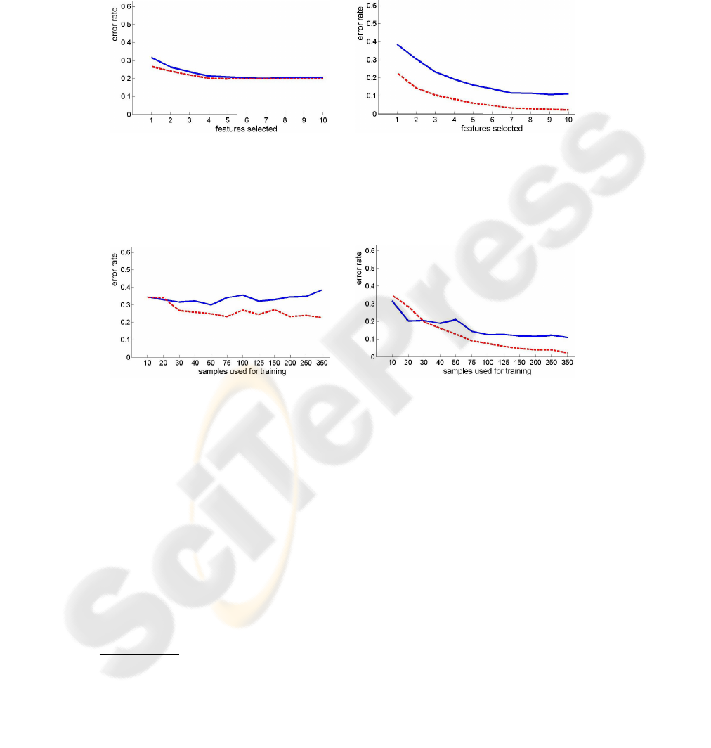
how the error rate depends on the number training samples. If we only choose the best
feature, we prune the tree of the strong classifier to much. Then, the error rates of
Adaboost and ADTboost are similarily bad. If we select more features, the error rates
decrease; and the difference between Adaboost and ADTboost enlarges, too.
Fig. 2. Error rates of Adaboost (solid blue line) and ADTboost (dashed red line), where the train-
ing step was based on 30 (left) and 350 (right) samples from the synthetic data set.
Fig. 3. Error rates of Adaboost (solid blue line) and ADTboost (dashed red line), where only the
best feature (left) and all ten features have been used for testing on the synthetic data set.
Experiments on Benchmark Data. For our experiments, we chose the four bench-
mark data sets breast cancer, diabetes, german and heart
1
, which have
been edited as two-class problems by [12]. Due to the limited space, we mainly present
the results of the breast cancer data set.
Our tests have a similar setup as the tests on the synthetic data. For each test, we
randomly selected up to 350 samples for training and testing. Then, we randomly sepa-
rated 100 samples (between 30% and 40% of the data) for testing, and the rest could be
used for training. Again, we repeated these tests 100 times. The breast cancer dataset
contains 263 samples of nine features. Some of the average error rates of our tests are
listed in tab. 1 and shown in figs. 4. We are very pleased that our lowest classification
errors is in the same range as the results of [12]. For the other two benchmark data
1
available at http://theoval.sys.uea.ac.uk/matlab/default.html
120

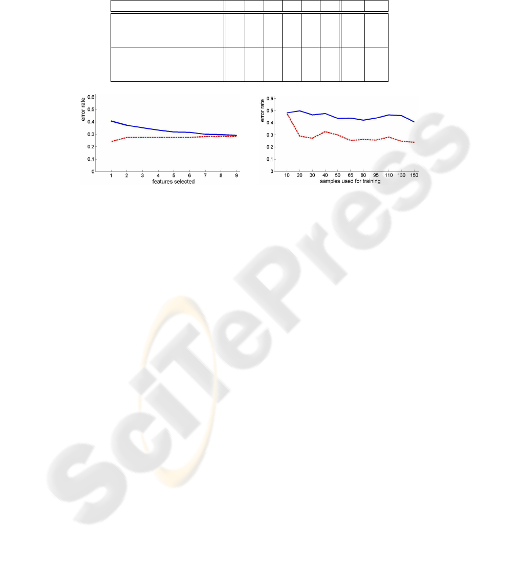
Table 1. Average error rates of breast cancer data set. The last two column refer to the results in
[12], where a single RBF classifier and Adaboost with more complex weak classifiers have been
used, respectively.
samples used for training 10 30 50 80 110 150 RBF AB
Adaboost, 1 feature selected 0.48 0.47 0.44 0.42 0.46 0.41
5 features selected 0.39 0.38 0.32 0.34 0.30 0.32
all 9 features 0.37 0.35 0.31 0.30 0.28 0.29 0.276 0.265
ADTboost, 1 feature selected 0.48 0.27 0.30 0.26 0.28 0.24
5 features selected 0.48 0.28 0.30 0.26 0.30 0.28
all 9 features 0.48 0.28 0.30 0.26 0.30 0.28 0.276 0.265
Fig. 4. Experiments on the breast cancer data set: Error rates of Adaboost (solid blue line) and
ADTboost (dashed red line), where the training step was based on 150 samples (left) or only the
best feature was selected (right).
sets, we obtain error rates which are not in the same range as in [12], but almost twice
as high. Thus, our linear weak classifiers are not suitable for these data sets. If the two
classes are badly separable by single-feature threshold classification, ADTboost either
favors weak classifiers with many preconditions, and their classification fraction con-
cerns only few samples, or the alternating decision tree is has almost no tree structure,
but contains many weak classifiers which share the same precondition.
The error rates of Adaboost decrease almost monotonously because of the reason-
able ranking of the weak classifiers. The tree structure of the strong classifier of ADT-
boost leads to complications when choosing a subset from it. We assume that the pruned
weak classifiers may have important effects on the classification result of several sam-
ples. If we have a tree with a large depth, any sensible feature selection scheme can lead
to bad classification results. We need to investigate the unexpected behaviour of ADT-
boost, showing increasing error rate when selecting more features. We assume that this
is due to the overfitting of ADTboost.
6 Conclusion and Outlook
We compared Adaboost and ADTboost with respect to our new proposed feature subset
selection method. So far, we implemented both classification techniques considering
only linear weak classifiers. Thus, we obtain reasonable and good results on synthetic
data and those benchmark data sets, where the linear classifiers are feasible. We are
121

mainly interested in interpreting images of man-made scenes, e. g. facade images of
building. We present our results of this real world data in [5].
We are going to improve our feature subset selection scheme. Therefore, we might
expand our feature space and look for more complex weak classifiers on 2-dimensional
feature planes as f
d
× f
2
d
. Furthermore, we want to extend it towards the multiclass
classification.
Acknowledgment
This work has been made within the project eTraining for Interpreting Images of Man-
Made Scenes (eTRIMS) which is funded by The European Union.
References
1. Chr. M. Bishop. Pattern Recognition and Machine Learning. Information Science and
Statistics. Springer, 2006.
2. L. Breiman. Random forests. Machine Learning, 45:5–32, 2001.
3. F. De Comit
´
e, R. Gilleron, and M. Tommasi. Learning multi-label alternating decision trees
and applications. In Proc. CAP 2001, pages 195–210, 2001.
4. M. Drauschke. Feature subset selection with adaboost and adtboost. Technical report, De-
partment of Photogrammetry, University of Bonn, 2008.
5. M. Drauschke and W. F
¨
orstner. Selecting appropriate features for detecting buildings and
building parts. In 21st ISPRS Congress, 2008 (to appear).
6. Y. Freund and L. Mason. The alternating decision tree learning algorithm. In Proc. 16th
ICML, pages 124–133, 1999.
7. I. Guyon and A. Elisseeff. An introduction to variable and feature selection. Journal of
Machine Learning Research, 3:1157–1182, 2003.
8. G. Holmes, B. Pfahringer, R. Kirkby, E. Frank, and M. Hall. Multiclass alternating decision
trees. In Proc. 13th ECML, LNCS 2430, pages 161–172. Springer, 2002.
9. H. Liu and H. Motoda. Feature Selection for Knowledge Discovery and Data Mining. Kluwer
Academic, 1998.
10. M. J. Martin-Bautista and M.-A. Vila. A survey of genetic feature selection in mining issues.
In Proc. CEC 1999, volume 2, pages 1314–1321, Washington D.C., USA, July 1999.
11. D. Mladeni
´
c. Feature selection for dimensionality reduction. In SLSFS, LNCS 3940, pages
84–102, 2006.
12. G. R
¨
atsch, T. Onoda, and K.-R. M
¨
uller. Soft margins for adaboost. Machine Learning,
43(3):287–320, March 2001.
13. J. Rogers and St. Gunn. Identifying feature relevance using a random forest. In SLSFS,
LNCS 3940, pages 173–184, 2006.
14. R. E. Schapire. The strength of weak learnability. Machine Learning, 5(2):197–227, 1990.
15. R. E. Schapire and Y. Singer. Improved boosting algorithms using confidence-rated predic-
tions. Machine Learning, 37(3):297–336, 1999.
122